
THE idea that we can divide music into two types, tonal and atonal, has often been contested, not least by the composer who created the defining compositional method associated with atonality, twelve-tone serialism. Arnold Schoenberg wrote that "the expression 'atonal music' is nonsense" (Simms, 2000, p. 8). Music psychology offers a potential resolution of this debate by defining tonality not as a property of music per se but as a mode of listening. We can listen to any music, including twelve-tone music, with tonal ears. What differs between musical pieces is the strength with which they enforce interpretation in a specific key.
Krumhansl, Sandell, and Sergeant (1987) showed that listeners could infer tonal contexts from twelve-tone rows with some consistency. Von Hippel and Huron (2020) ask the natural follow-up to this question: do composers actively work to encourage or discourage the hearing of tonal implications? Krumhansl, Sandell, and Sergeant's methodology immediately lends itself to an empirical method of answering this question, comparing row segments to Krumhansl and Kessler's (1982) tonal hierarchy. More recent research has continued to show that correlation with tonal key profiles is a good predictor of listener judgments of tonality (Anta, 2017). Von Hippel and Huron's results are musicologically interesting: in certain broad respects, they confirm what we might expect (Berg encourages tonal hearing, Webern discourages it), but they also provide additional nuance to those judgments. As a music theorist, my immediate reaction to their results is to ask how we can dig deeper: if these composers promote or obstruct tonal hearing, how do they do it? What aspects of tonality or atonality are they emphasizing? We know that tonality is more than a simple, unidimensional quantity (more tonal/less tonal). At a next approximation, tonality clearly has two dimensions, roughly equating to position of the scale on circle of fifths and of the tonic triad on the circle of diatonic thirds. Krumhansl and Kessler (1982) showed this using a multi-dimensional scaling procedure. The discovery of the multi-dimensionality of tonality accounts for the enormous influence of this study more than do its major and minor key profiles, even as these have become a ubiquitous yardstick in research on perception of tonality. After all, the probe-tone procedure and the idea of tonal profiles was not new, having been adopted from an earlier study by Krumhansl and Shepard (1979).
Further developing the concept of tonal space, Krumhansl (1990) notes that these two dimensions can be derived by a more purely mathematical procedure, the discrete Fourier transform (DFT) on pitch-class vectors, bypassing the more computational, complex data analysis method (multidimensional scaling) used by Krumhansl and Kessler (1982). This method of analyzing probe-tone data was also applied by Cuddy and Badertscher (1987). Much has been written recently to explain this procedure (e.g., Amiot, 2016; Quinn, 2006; Yust, 2016, 2017, 2019) which need not be fully recounted here. To give brief summary, the pitch-class vector turns a pitch-class set or distribution into a periodic signal, like (1,0,0,0,1,0,0,1,0,0,0,0) for the C major triad, and converts it into six periodic components, Fourier coefficients f1–f6. Each of these has a magnitude, indicating the presence of that periodicity and independent of transposition, inversion, and complementation, and a phase, indicating the orientation of the periodic component with respect to pitch-class zero. The two dimensions of tonality that Krumhansl and Kessler discovered correspond to the third and fifth Fourier coefficients. The nice mathematical properties of the discrete Fourier transform make this an especially expedient way to frame the questions that von Hippel and Huron ask, and to interpret their results. In particular, we can begin by asking, for example: If Berg encourages tonal hearing in his rows, does he do it through the medium of one dimension of tonality or the other? Or, if Webern discourages tonal hearing, is there a particular nontonal dimension that he favors in his practice? The answer to both questions, it turns out, is yes.
Krumhansl's observation can be demonstrated mathematically by applying the DFT to the tonal profiles. Figure 1 shows the spectra of the major and minor tonal profiles from Krumhansl and Kessler (1982), corresponding to the magnitudes of the six coefficients. In both cases, the most important coefficient is the fifth, the second most important is the third.
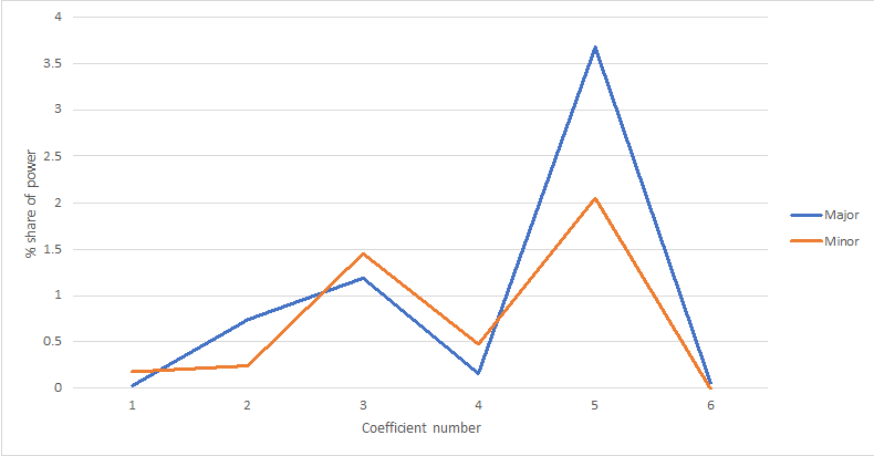
Figure 1. Spectra of Krumhansl and Kessler's (1982) tonal profiles
Tonal fit, following Krumhansl's work, is typically modeled by a correlation with these tonal profiles, or other similar ones. The Fourier transform has a nice property that helps us understand how these correlations work, established by the convolution theorem, which shows that the correlation of two pitch-class vectors is equivalent to a dot product of their Fourier coefficients. Therefore, the highest correlations will occur when (1) the two vectors have large values on the same coefficients and when (2) those large coefficients are aligned in phase. For the tonal profiles, this translates into: (1) tonal fits are higher for pitch-class sets or distributions with large third and fifth coefficients, and (2) the best fit is obtained by transposition of the major or minor keys to minimize phase differences of these coefficients. The second point means that the process of key finding can be understood in a tonal space (Krumhansl's toroidal space), with the phases of the third and fifth coefficients as the two dimensions. We can plot a pitch-class vector in this space using the DFT, and the nearest major or minor key in the space will be the best-fitting key for that pitch-class set or distribution. In Yust (2017), I show the conditions under which this procedure breaks down, which correspond to conditions of tonal ambiguity that we can classify using other elements of the DFT. Not surprisingly, we find all of these methods of achieving tonal ambiguity being used in the twelve-tone row data set under investigation.
The two dimensions of tonality correspond to musical properties that are easily observed in the major and minor profiles: (1) they favor pitches of the basic diatonic scale of the key, and (2) they favor pitches of the tonic triad. The first property leads to the dimension of diatonicity, represented by the fifth coefficient, and what we may for present purposes refer to as triadicity, represented by the third coefficient. More generally, this coefficient might be understood in reference to its prototype, the hexatonic scale, cf. Quinn, 2006. If a given tone row produces a relatively high tonal fit according to von Hippel and Huron's methodology, that might be because it favors diatonic sets, triadic sets, or some combination of the two.
The DFT also specifies a relatively small set of atonal dimensions. Since the energy of the "pitch-class signal" has to go into some periodicity, a set with a low tonal fit must have a correspondingly high "atonal" fit in this sense. The possible dimensions of atonality are: chromatic clustering (coefficient 1), tritonal clustering (coefficient 2) as would occur in, e.g., a chord built out of alternating perfect and augmented fourths, octatonicity (coefficient 4), and whole-tone balance (coefficient 6), the difference in weighting between the two whole-tone collections. We might notice from Figure 1, however, that two of these, tritonal clustering and octatonicity, are somewhat characteristic of the major and minor profiles, respectively. These are essentially mathematical artifacts: by not allowing for negative values, the probe-tone procedure essentially produces a "clipped" signal, and the clipping of a signal made from pure f3 and f5 components will produce a component corresponding to either the sum (f4) or difference (f2) of those. Distortion of this kind can be attributed to some extent to any pitch-class counting or rating procedure. The resulting artefacts are analogous to combination tones in audio. Which is more prominent depends upon the relative phases of f3 and f5, which is the primary difference between major and minor. Although we can understand the prominence of f2 and f4 in the tonal profiles as mathematical artefacts, they are not insignificant. For instance, the presence of these components will lead to higher correlations with the tonal profiles. While they can be understood as dimensions of atonality, they come with more constraints than f1 and f6. For instance, in the presence of a large f3 component, an f2 component at certain phase values will produce diatonicity (f5), so there are a limited range of phase values available to this component in an atonal context.
To summarize, then, we can say there are two tonal dimensions, f3 and f5, two principal atonal dimensions, f1 and f6, and two mixed dimensions, f2 and f4. The mixed dimensions are not necessarily inconsistent with tonality but can be atonal under the right circumstances. This gives us a simple classification of ways that a pitch-class set can be tonal or atonal.
Because the basic questions of von Hippel and Huron's research generalize over transposition, we can focus on DFT magnitudes, giving a relatively simple way to explore their data set to enhance their results, by taking the DFT of row segments and ignore the phase information. The DFT also provides a number of simplifications that make some of the aspects of their computational procedure unnecessary. Complementary sets have equivalent spectra, so the initial hexachord of a row will give exactly the same results as the final hexachord. Inversions also have equivalent spectra, so we need only investigate the prime forms. Given the limited scope of this response, and mindful of exhausting the statistical power of this small data set, I avoid doing too much additional hypothesis testing here, viewing this as an investigation primarily of the algorithm for determining tonal fit and its mathematics. However, some further questions about the statistical properties of the data set were ultimately prompted by the initial investigation, so one additional test is performed below.
To replicate von Hippel and Huron's results using the DFT, I tested a few methods of decreasing complexity and checked the rankings against theirs as if it were a ground truth. The first was to compare the spectra with the major and minor tonal profiles and take the highest value. This is not quite equivalent to correlating these as pitch-class vectors because there might be small differences in how good a match in phase values is possible, but since choosing the best-fitting key is equivalent to minimizing these phase differences, we can expect this variation to be small. The second measurement is a weighted sum of diatonic (f5) and triadic (f3) components, which is similar to the first method but simpler, in that other coefficients are ignored entirely. The third measure is just the diatonic component by itself, which we would expect to be too simplified to yield the same result, but shows exactly in which cases the triadic dimension plays an important role in the tonality of the row.
First, to check my assumption that the DFT spectrum provides an adequate substitute for von Hippel and Huron's procedure, I took the DFTs of the first and last dyads, trichords, tetrachords, and pentachords, and the initial hexachord of the row (by the complementation property, the two hexachords have the same spectrum), normalized these by power, 2 took the covariances with the power-normalized Krumhansl-Kessler major and minor spectra, chose the larger of the two for each set, and averaged these. The resulting ranking for the 86 rows was indeed very close to von Hippel and Huron's ranking, with a Spearman coefficient of .95. Of the set of top-15 rows mentioned by von Hippel and Huron, this procedure only misses the last two, which are the rows from Schoenberg's Op. 28/1 and Op. 29, the latter being a near miss (rank 16 instead of 15). The ambiguity of Op. 28/1, shown in Figure 2, is rather poetically appropriate, considering the text of the piece. This was ranked 22 by the DFT procedure, which instead preferred the "Akrobat" row from Berg's Lulu, shown in Figure 3 (rank 17 by von Hippel and Huron, and 10 by the DFT procedure). These discrepancies may be attributable to the discarding of phase information. The tonalness of Schoenberg's row is primarily attributable to the initial triad, which is able to neatly align in phase with multiple components. The tonalness of the Akrobat row is almost entirely in the dyads and (027) and (025) trichords. When these are phase-aligned with the f5 of a key, they are poorly aligned with the other important components, i.e., f2 and f3 or f4 and f3.
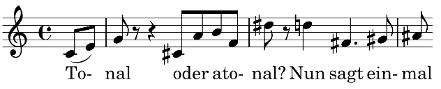
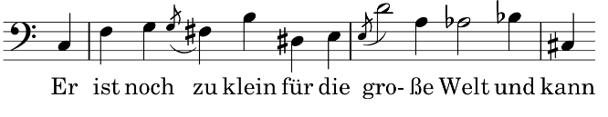
Figure 2. The rows from Schoenberg's Op. 28(1) (m. 1, top) and the "Akrobat" row from Berg's Lulu (Act II, mm. 100–103, bottom)
The phase information, therefore, while not completely insignificant, ultimately makes little difference overall. Ignoring it greatly simplifies the procedure: rather than check the correlations with twelve pitch-class weightings for 24 keys, we just check correlations of six values for two spectra. The greater simplicity of the procedure also might help simplify the hypothesized psychological mechanism. It is implausible that a listener would recheck fits with 24 keys with each new note. The process could be simplified by assuming only shifts to closely related keys need to be considered, but still, the procedure would often result in a very rapid series of modulations, where a new context is adopted to interpret each new note. The DFT-based method, on the other hand, only requires tracking and updating a small number of quantities. The DFT also lends itself to further simplifications. In particular, the major- and minor-key spectra are similar enough that we probably do not need to compare to both of them independently, and the covariance or correlations with these spectra are going to depend mostly on f3 and f5. Therefore, I also tried ranking the rows using only the quantity 2f̃32 + 3f̃ 52, where the notation f̃n2 refers to the power-normalized magnitudes (share of total power). The 2:3 weighting roughly splits the difference between major and minor. This continues to produce a ranking very close to von Hippel and Huron's results, with a Spearman correlation of .91 (and the match tends to be better for the more tonal rows, with weaker correlation in the low-ranked rows). Again, the top 15 rows are only different by two, Schoenberg's "Tonal oder atonal" (Op. 28/1) and the Alwa row from Lulu (ranked 11 by von Hippel and Huron, 18 by 2f̃32 + 3f̃ 52). The latter, shown in Figure 3, is similar to "Tonal oder atonal" in that it begins with a consonant triad and ends with some relatively atonal sets.
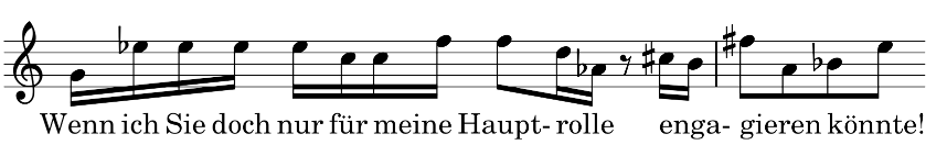
Figure 3. Alwa's row from Lulu (Act 1, mm. 98–99)
We can also get a reasonable measure of tonal fit with f̃ 52, diatonicity, alone. The average of the nine f̃ 52 values for each row agrees with von Hippel and Huron's with a 0.71 Spearman correlation. Remarkably, this ranking still identifies 13 of von Hippel and Huron's top 15. This suggests that diatonicity is the primary way for Berg in particular to construct rows with tonal implications. It partially reflects the mathematical fact that f5 is the single coefficient most important for tonality, but also tells us something about the data set, namely that diatonicity in absence of triadicity is more prevalent than the reverse. In principle, discrepancies between diatonicity and correlation with a key profile are relatively easy to produce, and we can find some examples in the data set. Figure 4 shows two instances where the f̃ 52 criterion is very different from the other two. Schoenberg's Op. 29 uses the hexatonic scale (a pure representative of f3) as its hexachord. The large |f3|s lead to a relatively high ranking (15) by von Hippel and Huron's method, but it drops to the basement (74) when the criterion is f̃ 52. At the same time, Schoenberg's Op. 33b, whose primary quality is whole tone, ranks fairly highly on f̃ 52 (number 10), while it is much farther down (number 45) on von Hippel and Huron's list. The sets of the row are consistently diatonic, or nearly so, but mostly with scalewise sets that avoid triads and triadic subsets.
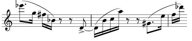
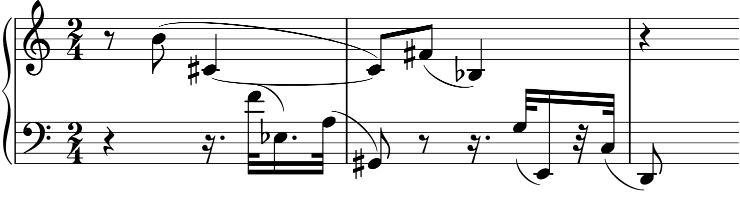
Figure 4. Rows from Schoenberg's Op. 29 Suite (mm. 11–13, top) and Op. 33b Klavierstuck (mm. 1–3, bottom).
Having established this initial proof of concept, let us look more closely at the questions that the DFT enables us to answer: Which dimensions of tonality and atonality are most important for different composers' choices of rows? To amplify the musicological value of this analysis, I added some non-Viennese rows to von Hippel and Huron's data set, 18 rows used by Stravinsky in his late works. 3 On all of the tonality ranking procedures just described, Stravinsky's rows are generally quite low, similar to Webern's, with one exception, the row from Anthem ("A Dove Descends Breaking the Air") which is in the top ten on all measures.
To see whether specific harmonic qualities (Fourier coefficients) are characteristic of each of the four composers' rows, I averaged all the power-normalized coefficient sizes for each row, and ran a one-way ANOVA by composer for each component. Table 1 shows the results, with raw p values. A Bonferroni-corrected standard α gives a p < .008 criterion, which is met only by f1 and f5, although f3 and f6 give marginal values that look like they might well reach significance on a larger data set. Figure 5 plots spectra averaged across each composer's rows. 4
The f5 result is due to high diatonicity in Berg's rows and low diatonicity in Webern's. We do not see a similar difference in f3—in fact, if anything, Webern tends to have higher f3s than the other composers. The distinction in tonal fit between the Viennese composers is therefore attributable to diatonicity. The other significant result (on f1) is that Webern and Stravinsky use rows with higher chromatic clustering. In particular, we may note that these two composers differ from Schoenberg in their preferred atonal dimension. Schoenberg tends to achieve atonality with whole-tone sets (high |f6|), while Webern and Stravinsky do so with chromatic concentration. The results are consistent if we look at spectra for just the initial and final tetrachords or the hexachords averaged across composers, as Figure 6 shows.
| Coefficient | MS | F | p |
|---|---|---|---|
| f̃ 12 | 1.89 | 12.62 | < .01 |
| f̃ 22 | 0.05 | 0.35 | — |
| f̃ 32 | 0.37 | 3.52 | .02 |
| f̃ 42 | 0.06 | 1.20 | — |
| f̃ 52 | 0.89 | 9.83 | <.01 |
| f̃ 62 | 1.28 | 3.14 | .03 |
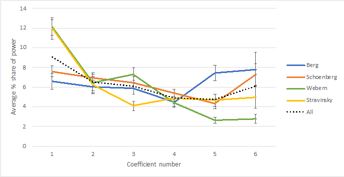
Figure 5. Average spectra by composer (bars: standard error)
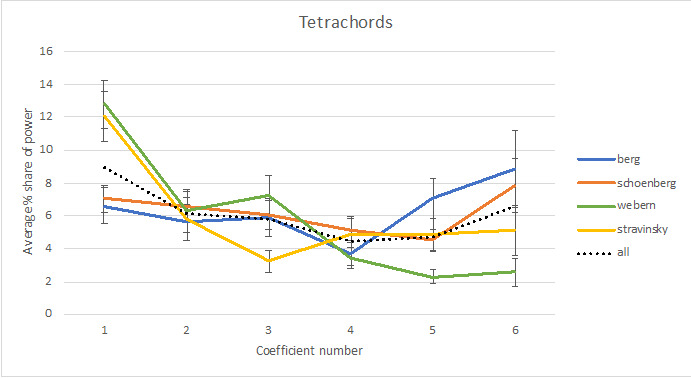
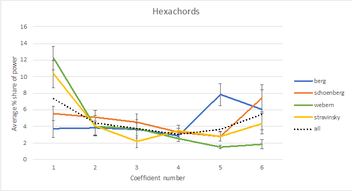
Figure 6. Average spectra for initial and final tetrachords (top) and hexachords (bottom) for each composer
The tonal implications of Berg's rows thus come, on the whole, from the diatonic implications of the initial and final sets rather than from triadic implications. We can also see notable consistencies in Webern's practice: the atonality of his rows is primarily accomplished by the use of chromatically clustered sets (f1), not whole-tone sets (f6). Whole tone quality actually has the lowest average across his data, in contrast to Schoenberg, who appears to favor whole-tone-weighted sets, at least in his hexachords. The distinctive aspect of Stravinsky's rows appears to be the avoidance of triadic/hexatonic quality (f3). His rows are similarly atonal to Webern's. We see no consistent differences in the use of the mixed qualities, f2 and f4, across composers.
We can check these results by composer by looking at the maximally atonal sets ranked by a combination of f1 and f6, a counterpart to the list of most tonal rows. Since the maximum possible |f6| is typically about twice the maximum |f1|, to avoid overweighting the former, I ranked the rows by 2f̃ 12 + f̃ 62. Even with the preferential weighting of f1, whole-tone-based rows remain a good strategy for maximizing atonality, because sets with maximal chromatic clustering have minimum |f6|, whereas it is possible to maximize |f6| and still have a relatively large |f1| on smaller-cardinality sets. For this reason, maximum atonality is actually more of a characteristic of Schoenberg, who accounts for seven of the top-20 (17% of his 42 rows) atonal rows by this criterion, and even more so of Stravinsky, who also has seven (39% of his 18 rows) in this top 20. Even Berg has more highly atonal rows than Webern according to 2f̃ 12 + f̃ 62; both have three in the top 20, but Berg's three are all in the top-10 (numbers 1, 2, and 6, all rows from Lulu: the "whole-tone" row, the Schigolch row, and the Schoolboy row), whereas Webern's are not (numbers 12, 13, and 19). The list of 20 includes a mixture of high-|f6| and high-|f1| rows, and the 2f̃ 12 + f̃ 62 criterion agrees fairly well with von Hippel and Huron's rankings for the most atonal rows (Spearman correlation of –.61). The top-15 non-Stravinsky rows include von Hippel and Huron's 7 least tonal rows. Only when we rank rows by chromatic clustering, f̃ 12, as a measure of atonality, does Webern stand out. Of the top 20 rows by f̃ 12, eight are Webern's (38% of his 21), and the same number, eight, are Stravinsky's (44%). Berg has only one on the list, the Schigolch row, but it is also the one with the highest f̃ 12 of the entire dataset. The remaining three are Schoenberg's (7%).
Figure 7 shows the row from Schoenberg's Op. 48/3, an example of a whole-tone row that ranks highly on 2f̃ 12 + f̃ 62 (number 8), and is the least tonal by von Hippel and Huron's criterion. It also has the lowest f̃ 12 of the entire data set.
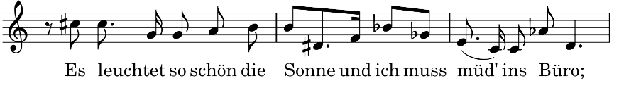
Figure 7. The row from Schoenberg's Op. 48/3, mm. 3–5
Figure 8 shows the row for Webern's Op. 21, an example of a row that is high both on f̃ 12 and 2f̃ 12 + f̃ 62 (number 4 and 12 out of 104 respectively) due to the use of chromatic tetrachords and hexachords. By von Hippel and Huron's method, however, it gets a moderately tonal ranking (number 41) because of its use of thirds particularly at the beginning and end.
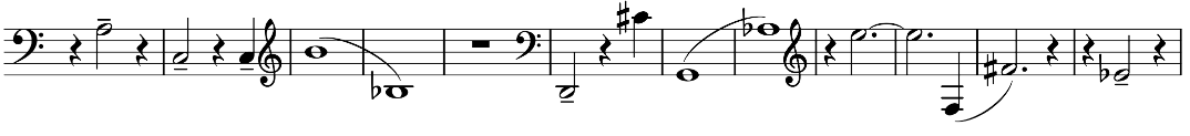
Figure 8. The row for Webern's Op. 21, mm. 3–14
The findings presented here, like those of von Hippel and Huron, are not entirely surprising. Analysts have often noted the importance of semitones and chromatic sets for Webern, whole tone sets for Schoenberg, and diatonic sets for Berg. The value of von Hippel and Huron's work is in quantifying these observations and backing them up with data. My extension of their results has a somewhat different kind of value, I would argue. By reframing the idea of tonal fit using harmonic qualities, I simplify it and at the same time show that it has non-trivial dimensionality and that these composers do not treat the two dimensions of tonality equally. High tonal fit in twelve-tone rows is usually achieved through diatonic sets (f5) rather than triadic ones (f3). Furthermore, because the number of possible harmonic qualities is quite limited, composers seeking non-tonal harmonic material have very limited options. Of the two simplest and most direct options, chromatic clustering (f1) and whole-tone sets (f6), the former is preferred by Webern and the latter by Schoenberg.
ACKNOWLEDGEMENTS
This article was copyedited by Niels Christian Hansen and layout edited by Kelly Jakubowski.
NOTES
- Correspondence can be addressed to: Dr. Jason Yust, Boston University, 855 Commonwealth Ave. Boston MA, 02215. Email: jyust@bu.edu
Return to Text - Specifically, I squared the magnitudes and divided by the sum of squared magnitudes, which is a constant for the cardinality.
Return to Text - These are all the rows that can be found in Kuster (2000), which includes most of the interesting examples. I used this source purely for convenience; a check of his analyses against row forms from my own in-depth analyses of four of the works showed perfect agreement.
Return to Text - The differences in f̃ 62 shown in Figure 5 are similar to those in f̃ 52, but the latter reaches significance because of its smaller variance. There is a mathematical reason for the high deviations in f̃ 62. For pitch-class sets, it is a coarse measure, taking only integer values. For instance, a trichord can only take four possible |f6| values, ±1 or ±2. The range of |f5| values is similar, but with many more finer distinctions possible.
Return to Text
REFERENCES
- Amiot, E. (2016). Music through Fourier space: discrete Fourier transform in music theory. Cham, Switzerland: Springer. https://doi.org/10.1007/978-3-319-45581-5
- Anta, J. F. (2017). Pitch dispersal and the perception of tonal strength in Schoenberg's oeuvre. Music Perception, 34(5), 541–56. https://doi.org/10.1525/mp.2017.34.5.541
- Cuddy, L. L., & Badertscher, B. (1987). Recovery of the tonal hierarchy: some comparisons across age and levels of musical experience. Perception & Psychophysics, 41, 609–20. https://doi.org/10.3758/BF03210493
- von Hippel, P., & Huron, D. (2020). Tonal and 'anti-tonal' cognitive structure in Viennese twelve-tone rows. Empirical Musicology Review, 15(1-2), 108-118. https://doi.org/10.18061/emr.v15i1-2.7655
- Krumhansl, C. (1990). Cognition foundations of musical pitch. New York, NY: Oxford University Press.
- Krumhansl, C. L., & Kessler, E. J. (1982). Tracing the dynamic changes in perceived tonal organization in a spatial representation of musical keys. Psychological Review of General Psychology, 89, 334–68. https://doi.org/10.1037/0033-295X.89.4.334
- Krumhansl, C. L., & Shepard, R. N. (1979). Quantification of the hierarchy of tonal functions within a diatonic context. Journal of Experimental Psychology: Human Perception and Performance, 5(4), 579–94. https://doi.org/10.1037/0096-1523.5.4.579
- Krumhansl, C. L., Sandell, G. J., & Sergeant, D. C. (1987). The perception of tone hierarchies and mirror forms in twelve-tone serial music. Music Perception, 5(1), 31–77. https://doi.org/10.2307/40285385
- Kuster, A. (2000). Stravinsky's topology: an examination of his twelve-tone works through object-oriented analysis of structural and poetic-expressive relationships with special attention to his choral works and Threni. Retrieved on 6th February 2020 from https://sites.google.com/site/stravinskystopology.
- Quinn, I. (2006). General equal-tempered harmony. Perspectives of New Music, 44(2)–45(1), 114–159 and 4–63.
- Simms, B. R. (2000). The atonal music of Arnold Schoenberg, 1908–1923. New York, NY: Oxford University Press. https://doi.org/10.1093/acprof:oso/9780195128260.001.0001
- Yust, J. (2016). Special collections: renewing set theory. Journal of Music Theory, 60(2), 213–262. https://doi.org/10.1215/00222909-3651886
- Yust, J. (2017). Probing questions about keys: tonal distributions through the DFT. In O. A. Agustín-Aquino, E. Lluis-Puebla, & M. Montiel (Eds), Mathematics and computation in music, 6th international conference, MCM2017 (pp. 167–182). Cham, Switzerland: Springer. https://doi.org/10.1007/978-3-319-71827-9_13
- Yust, J. (2019). Stylistic information in pitch-class distributions. Journal of New Musical Research, 48(3), 217–231. https://doi.org/10.1080/09298215.2019.1606833
