THIS paper investigates the processes leading to fame (for the few) or obscurity (for the many) in the world of music, whether for composers, performers, or works themselves. It starts from the observation that the patterns of success, across many historical music datasets, follow a similar mathematical relationship. The paper is intended for a musicological readership, and the mathematics have been kept to a minimum.
Let us begin with a simple exercise. Find a book, website or other source that lists composers or performers and says something about them or their music. You might choose a biographical dictionary; perhaps one of the many record guides; the catalogue of a music publisher or library; or an encyclopedia of jazz, pop, or opera. Or something else: the choice is yours.
Browse through your source – either methodically, or at a few random places – and pay attention to the lengths of the entries, which might be biographical articles, lists of works or recordings, or perhaps a combination. There will probably be many short entries about unfamiliar characters, but also a fair number of long entries about the big names. If your source is a book and you open it at random, there is a good chance that you will stumble across a major figure (e.g., Bach or Beethoven) simply because they occupy so much space in the book.
This is hardly unexpected, although you might be surprised at the number of short entries. If you examine the distribution of article lengths in detail, you may well find that they follow a mathematical pattern known as a power law. As we shall see, power laws are commonly found in music history, particularly in measures quantifying success, whether that means fame, productivity, exposure, sales volumes, desirability, or critical acclaim.
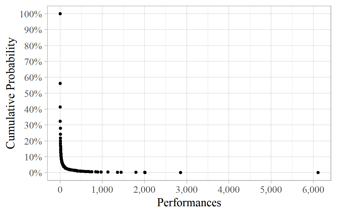
To illustrate the point, let us examine the BBC Proms Archive, 2 a listing of all Promenade concerts since 1895, and count how many times each composer has appeared. Using the data up to the 2015 season, I found around 58,000 entries (one for each performance of each piece) by almost 2,500 composers. The most performed were Wagner (6,100 performances), Beethoven (2,900), Mozart and Tchaikovsky (each about 2,000). Almost 1,100 composers (44% of the total) appeared just once. 3
Figure 1 illustrates this data graphically. It shows the proportion of composers (on the vertical axis) with at least the number of performances shown on the horizontal axis. Thus, top left, 100% of composers had at least one performance, and 56% had at least two (i.e., 100% minus the 44% with exactly one). Wagner, with 6,100 performances, is represented by the dot on the far right. The proportion of composers falls off very rapidly as the number of performances increases, and the fortunes of the big-name composers are extreme compared to the majority. The average number of performances is about 23 (i.e., 58,000 performances divided by 2,500 composers), although this does not represent a typical composer: 90% of composers had fewer appearances than this.
This shape is characteristic of a power law: it falls off steeply on the left, with a long tail to the right, covering a very wide range (1 to 6,100 in this case). For power laws, the average is rarely useful.
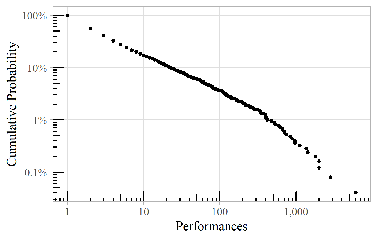
To confirm this as a power law we can plot the same graph using logarithmic scales. Figure 2 is similar to Figure 1, but with logarithmic scales, meaning that the intervals on each axis increase multiplicatively, rather than additively. 4 On the horizontal axis in Figure 2, each major tick (1, 10, 100, etc.) multiplies the previous value by 10, whereas in Figure 1 it adds 1,000. On such a "log-log plot", a power law reveals itself as a straight line.
The log-log plot is thus useful for identifying a power law, but also for making clearer the many points that otherwise bunch in the bottom left corner. We can now see, for example, that 4% of composers have had 100 or more appearances, which is impossible to determine from Figure 1.
Power laws are so named because the probability of getting a value x is inversely proportional to x raised to the power of a constant a, known as the exponent. 5 Mathematically, the probability p(x) is proportional to 1/xa. The exponent a is a measure of the slope of the straight line on a log-log plot. For the BBC Proms data, the exponent is about 1.9. 6
MORE POWER LAWS
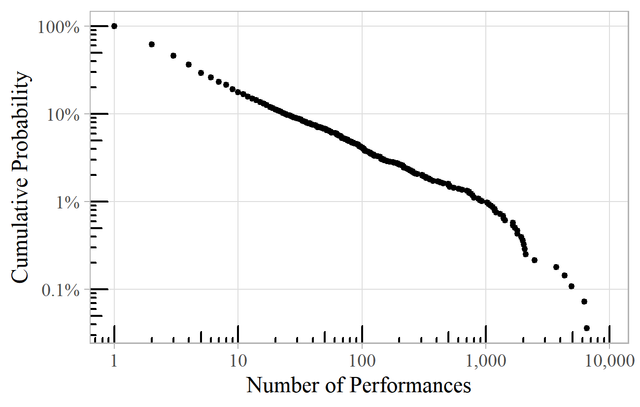
The BBC Proms example is by no means an isolated case. A similar chart emerges for the New York Philharmonic's concert history (Figure 3), 7 with an exponent of about 1.8. 8 In this case, Beethoven comes out on top, with Wagner just in second place.
A similar analysis can be done of the number of performances of individual works rather than of composers. These are also approximate power laws, with exponents of 2.9 for the BBC Proms (Figure 4) and 2.1 for the New York Philharmonic. Wagner's Tannhäuser (not necessarily in its entirety) leads the way at the BBC Proms, whilst Handel's Messiah is the most performed work by the New York Philharmonic.
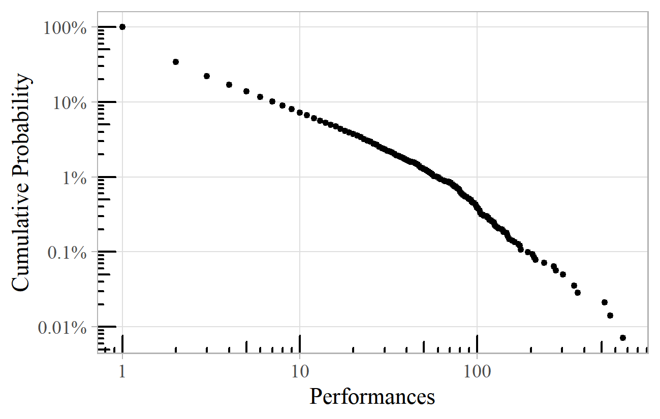
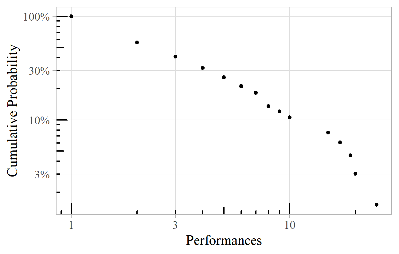
A power law may also apply to subsets of the data. The number of performances of Haydn symphonies at the BBC Proms also follows an approximate power law, with an exponent of 2.2 (Figure 5). Symphony No. 88 leads the way with 25 performances, followed by No 102 (20 performances), and No. 104 (19 performances). Twenty-nine have had just one Proms performance, and 38 of Haydn's 104 symphonies have had no Proms performances at all. 9
If we only knew about the BBC Proms performances, could we say anything about how many other Haydn symphonies had never appeared at the BBC Proms? In other words, could we extrapolate the power law to the left to estimate the number of symphonies with zero performances? Extrapolation is a dangerous procedure, so this is not to be recommended. Nevertheless, if we take the liberty of including the 38 unperformed symphonies in the data, and plot them at 0.5 on the horizontal axis (perhaps arguing that values up to 0.5 would be rounded down to zero), then it is intriguing that we still get the straight line of a power law. (We cannot plot them at zero, as the logarithm of zero is not defined). This suggests that it might be possible in some circumstances to extrapolate from the distribution of observed works, to estimate (somewhat speculatively) the number of unknown ones.
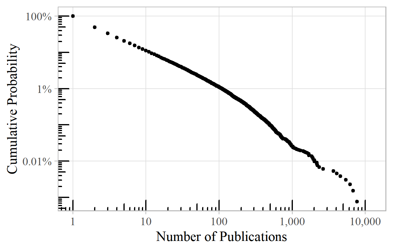
Printed music also shows power law behavior. Figure 6 plots the number of publications per composer among the million or so items in the British Library's music catalogue. 10 This roughly follows a power law with an exponent of 2.2.
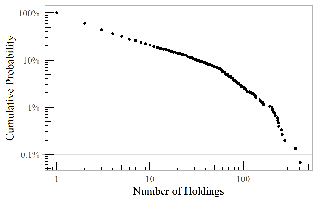
A similar pattern is revealed with the number of holdings of individual folk songs in the Vaughan Williams Memorial Library (Figure 7). 11 The exponent here is about 1.8.
Figure 8 shows the number of works per composer from a sample from Franz Pazdírek's (1904-1910) Handbook of Musical Literature cataloguing all printed music available, worldwide, in the early years of the twentieth century. The exponent is 1.8.
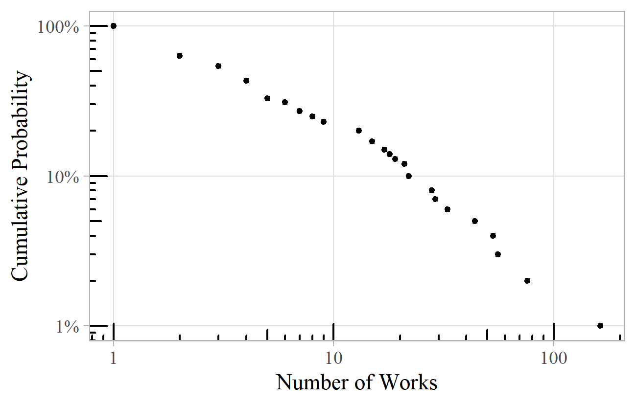
Figure 8. Works per Composer from a sample of 100 composers from Pazdírek's (1904-1910) Handbook of Musical Literature.
The online sheet music repository International Music Score Library Project (IMSLP) reveals similar patterns, and an example is shown in Figure 9: the number of works for each of the 800 or so female composers on IMSLP, giving a power law with exponent around 2.2. 12 IMSLP has a "random page" feature, which facilitates sampling from the whole dataset. The number of times each composer appeared in a sample of about 30,000 random works is distributed as a power law with exponent 2.4.
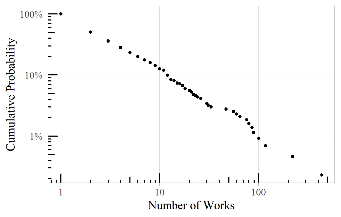
Figure 9. Number of works per female composer listed in the International Music Score Library Project (IMSLP).
Moving on to recorded music, the distribution of the number of recordings per work based on samples from several editions of the Penguin Record Guide (Greenfield, Layton, & March, 1975, 1988, 1999, March, Greenfield, Layton, & Czajkowski, 2007) is shown in Figure 10. 13 The exponents range from 1.9 to 2.3.
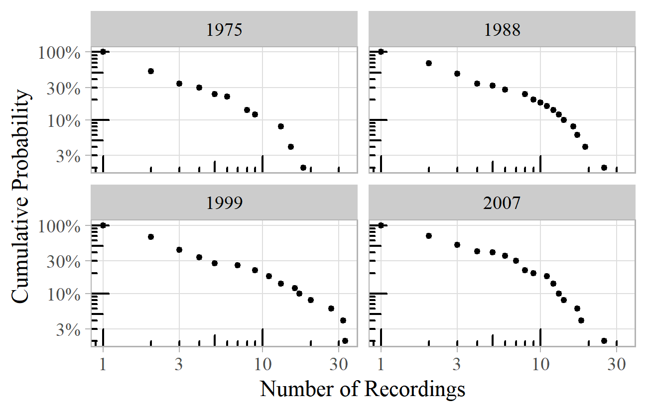
Figure 10. Recordings per work for several Penguin Record Guides (Greenfield, Layton, & March, 1975, 1988, 1999; March, Greenfield, Layton, & Czajkowski, 2007).
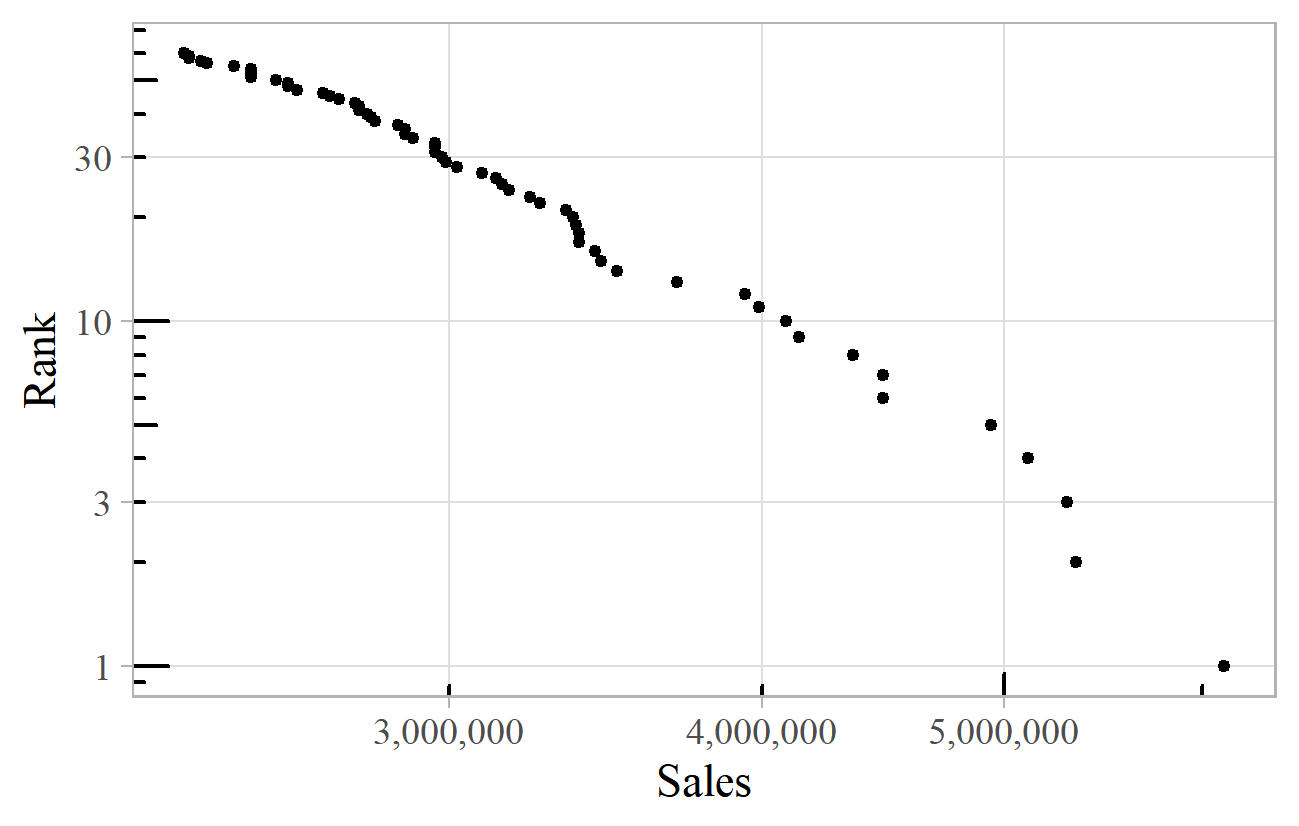
In popular music, power laws have been found in the number of gold records per artist (Cox Felton, & Chung, 1995), market shares of "Billboard Hot 100" singles (Haampland, 2017), the evolution of tracks in emerging genres (Keuchenius, 2015), the popularity of streamed songs (Krueger, 2019, pp. 86-91), and the listening habits of users of last.fm (Koch & Soto, 2016). Figure 11 shows a chart of UK all-time top 60 album sales. 14 This has a rather larger exponent than we have seen so far, 4.8, although this estimate is based only on the extreme end of a much larger distribution of all album sales, the data for which is not readily available. A similar high exponent is found for the chart of million-selling UK singles. 15
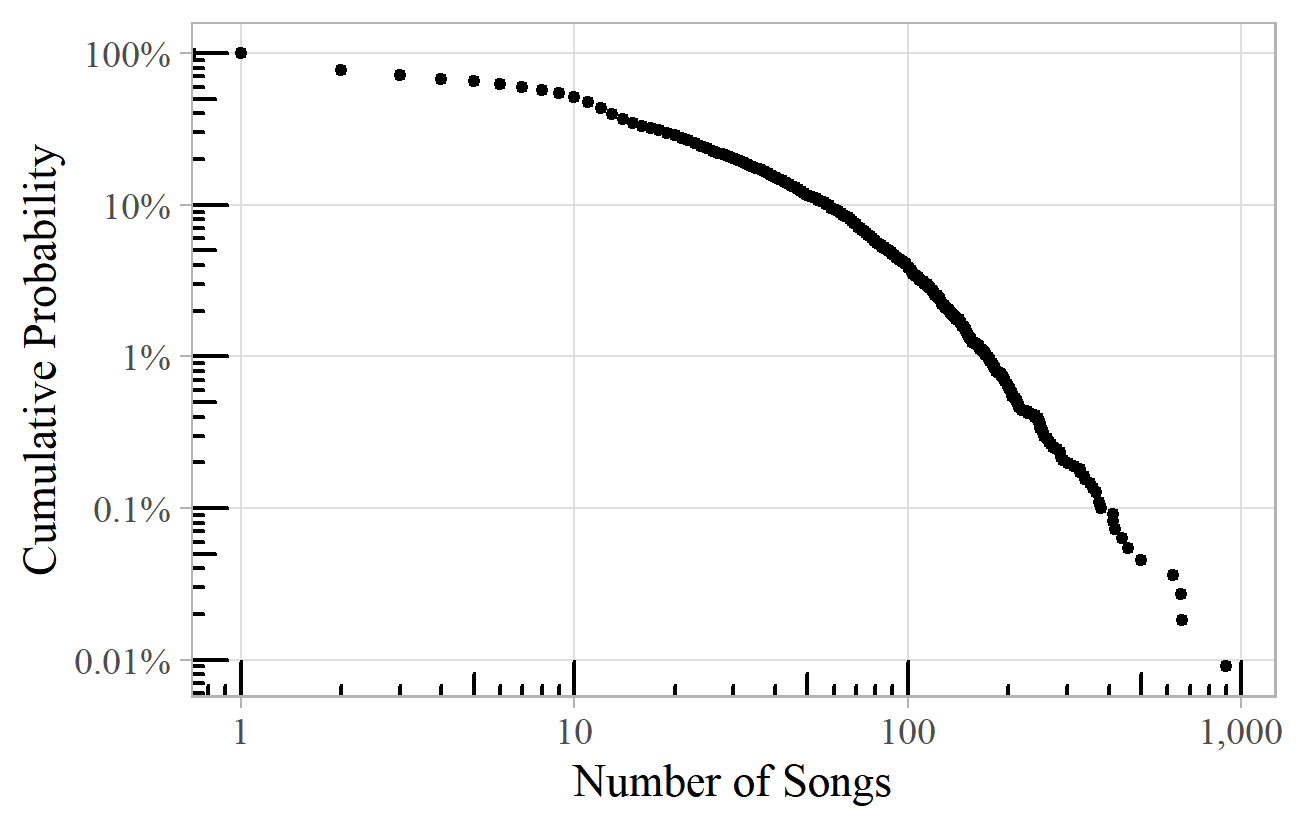
Figure 12 shows the distribution of songs per popular artist listed on the "Music Lyrics Database" website. 16 This is a less convincing straight line, especially the flat section for low numbers of songs, which might be because most artists will be represented by at least an album of perhaps ten songs. This sort of curved line may be better described by a lognormal distribution rather than a power law. The two are closely related, and they can arise in similar ways. The lognormal distribution is so called because the logarithm of the variable (the number of songs, in this case) is distributed according to the familiar bell-shaped normal distribution. It too can have a very long tail on the right, but on a log-log plot is often flatter on the left, usually with a gentle downward curve.
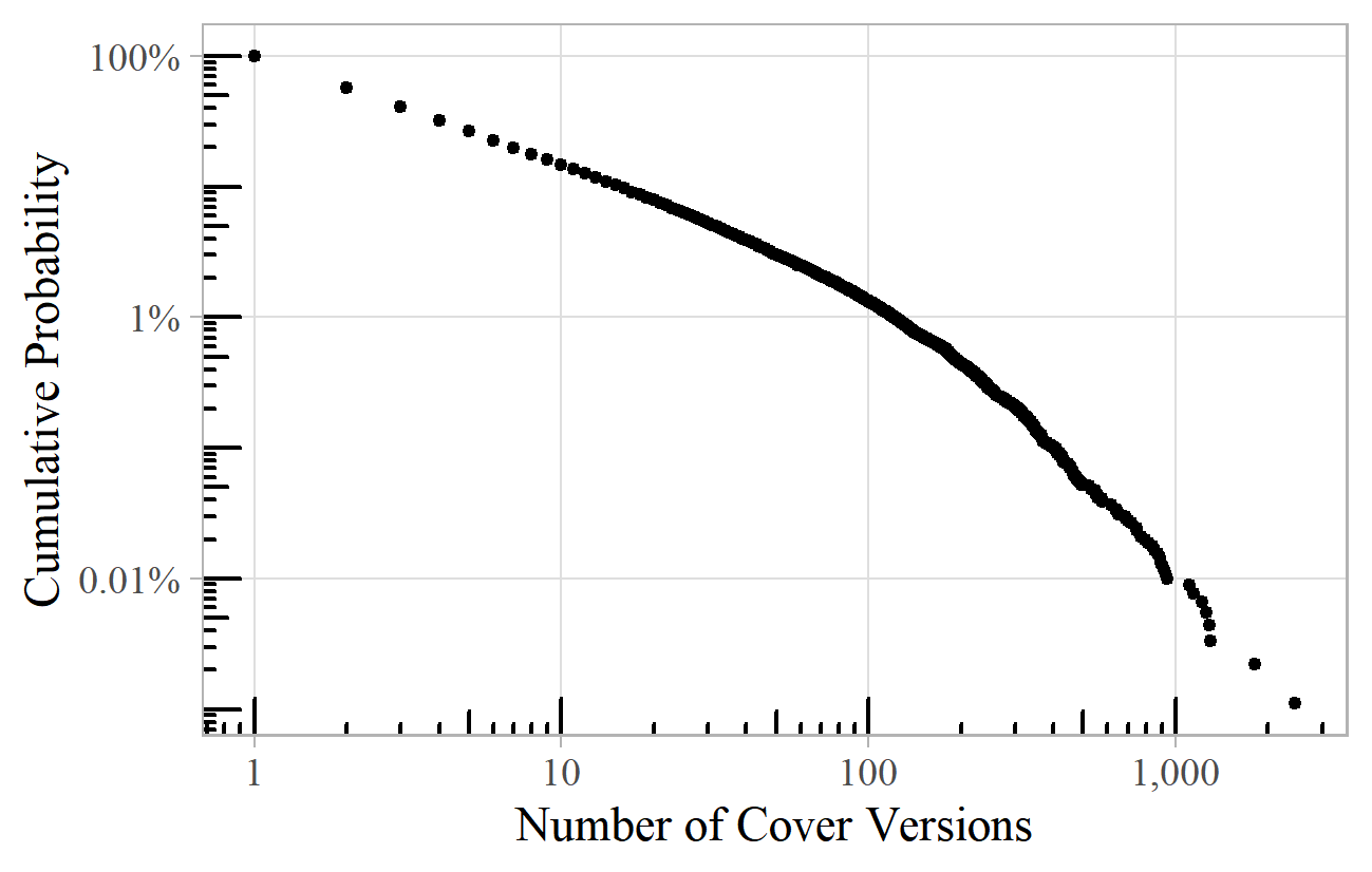
Figure 13 shows the power law distribution of the number of cover versions of popular songs, as listed on the "Second Hand Songs" website, with "Silent Night" on top with over 2,000 covers, and Gershwin's "Summertime" in second place. 17 The exponent here is about 2.0.
Power laws also describe auction prices paid for rare records. The website "Value Your Music" collects data for several formats and genres, and the distribution of the top 1,000 prices is shown in Figure 14 for vinyl records in total (top left) and the separate categories of classical, jazz and rock. 18 These have exponents between 3.3 and 4.2. As with the Haydn symphonies, the subsets of individual genres follow power laws within a similar distribution for the population as a whole.
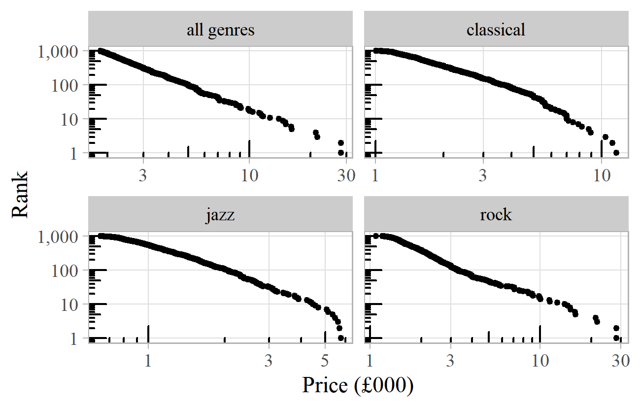
Figure 14. Top 1,000 auction prices for rare vinyl records according to the "Value Your Music" website.
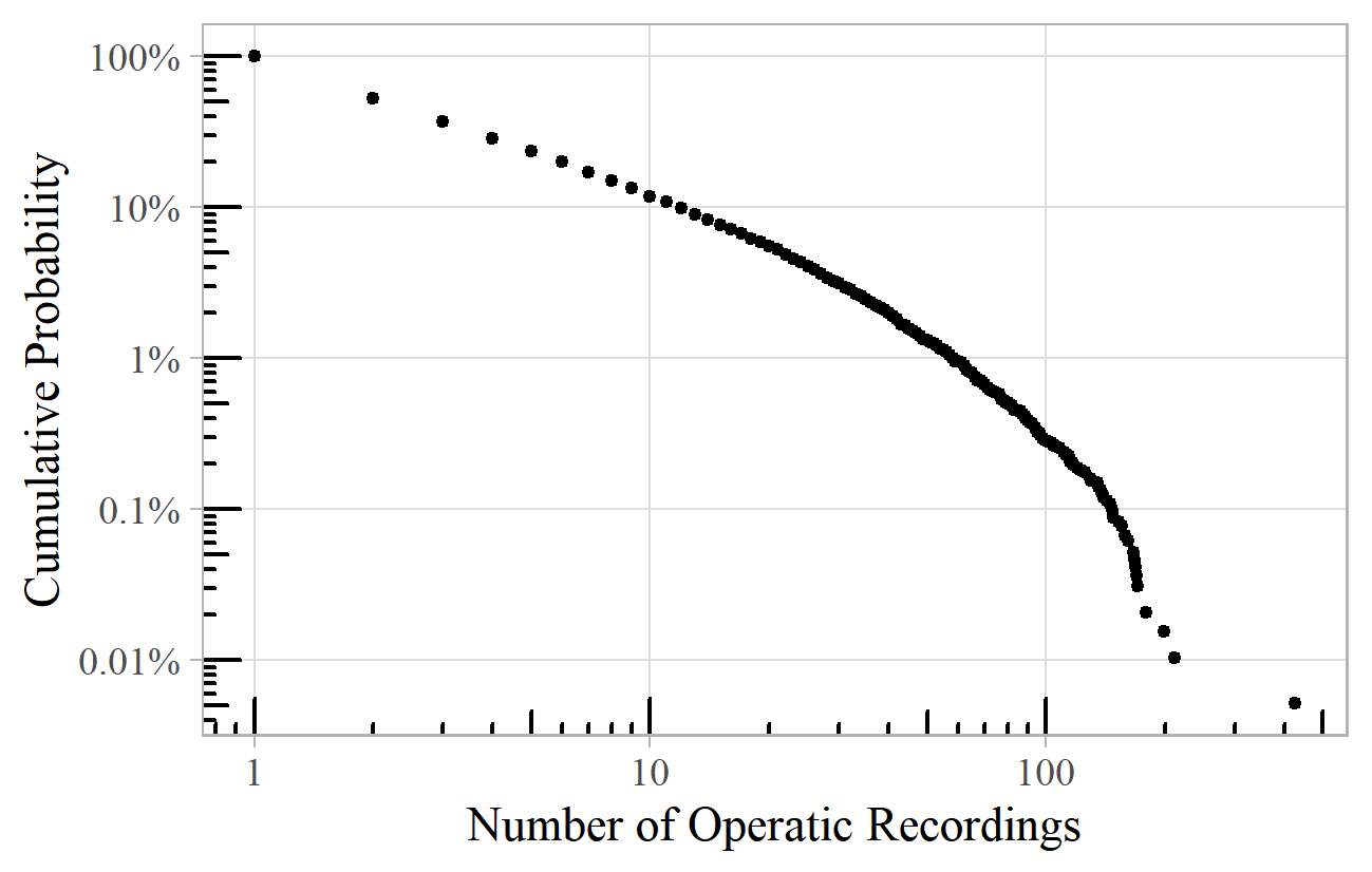
Power laws appear in the relationship between recordings and performers. Figure 15 shows the number of opera recordings in which individual singers have been credited. 19 The exponent here is about 2.2. This power law breaks down on the right. It is not uncommon for power laws to deviate from a straight line at the ends of the range. At the bottom, data might be censored if obscure works are unknown or omitted through a lack of space or interest. At the top end, there are often practical limits, such as how many recordings one singer can realistically undertake in a lifetime. The individual who breaks this barrier on the far right of Figure 15 is Placido Domingo, with more than twice as many recordings (426) as his nearest rival Montserrat Caballé.
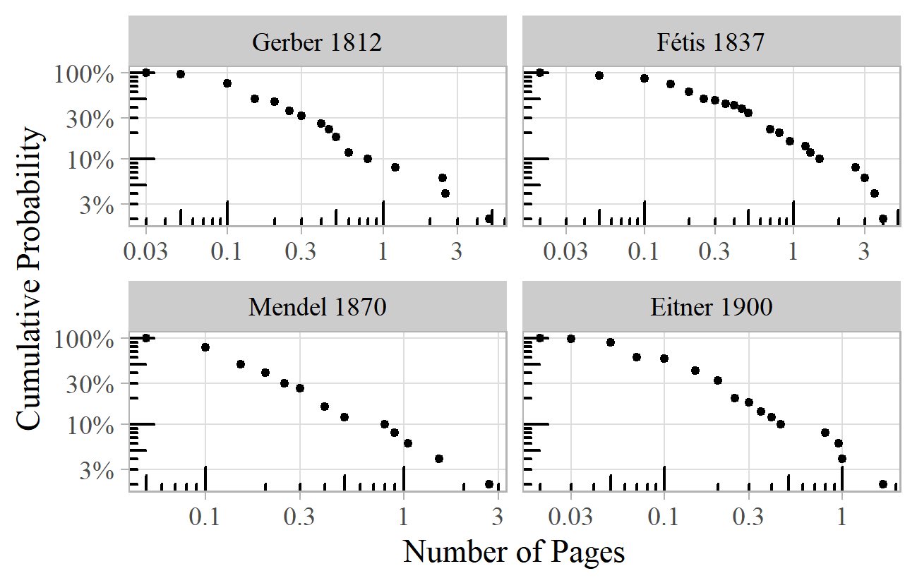
Even writing about music has power law characteristics. Biographical dictionaries have article lengths that follow this pattern. Figure 16 shows the article lengths for samples from four major European nineteenth-century biographical dictionaries. 20 The exponents range from 1.8 (Fétis) to 2.3 (Mendel). Whilst Mendel (bottom left) has a good straight line throughout, very short articles are underrepresented in the other sources, which might be better described by a lognormal distribution. This could be due to censoring of unknown or obscure names as discussed above.
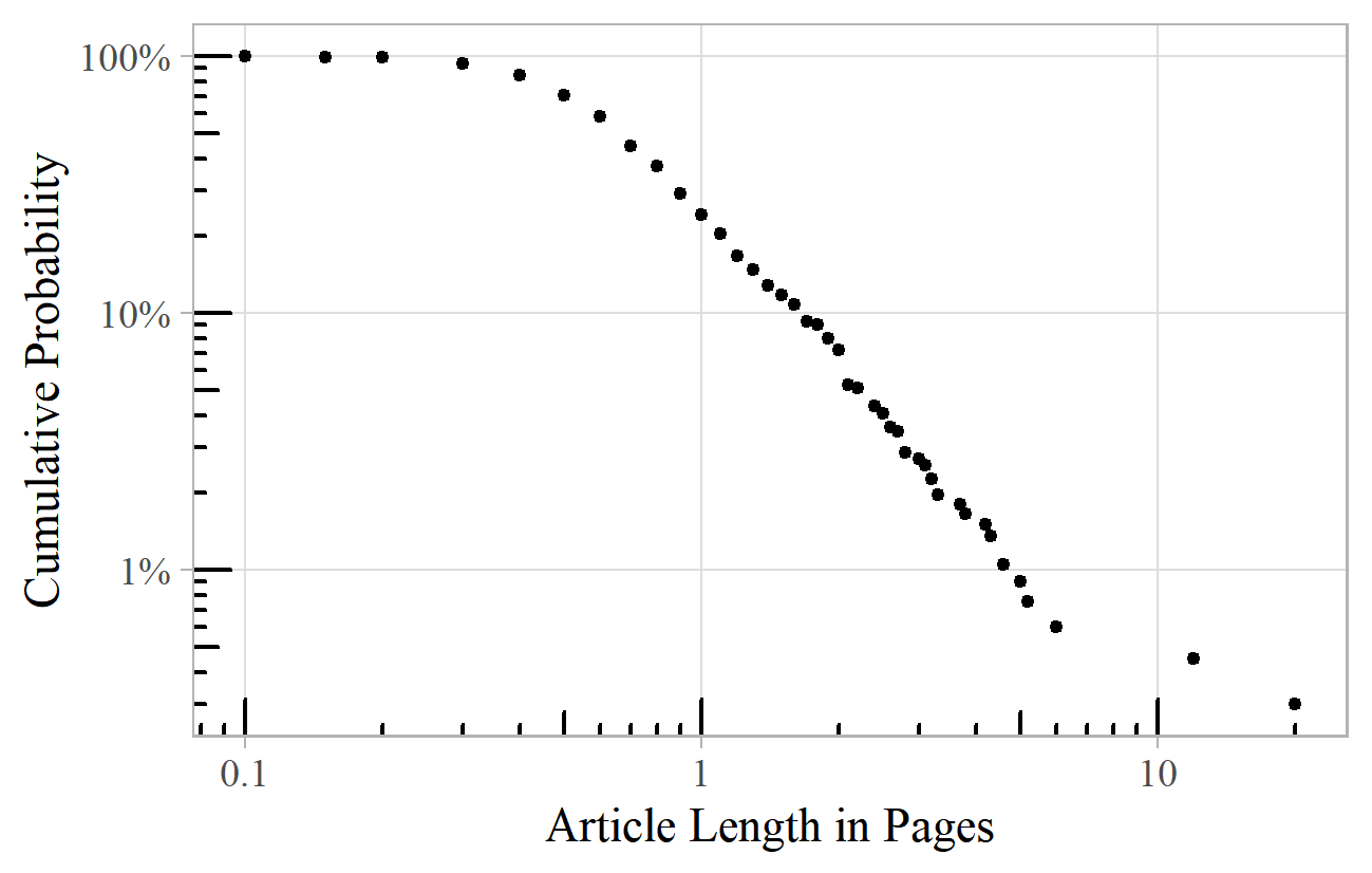
Oxford Music Online shows a lognormal-like distribution of article lengths (Figure 17). 21 Between half a page and six pages there is a nice straight line (with exponent of about 2.5), but shorter and longer articles do not fit the pattern. There is perhaps little point in very short articles, so the distribution is censored at this end. For long articles, there may be distortion due to the sampling method. Plotting this data as a histogram, with bands of log(article length) on the x-axis, and bar heights equal to the number of articles in each band, we do indeed see the familiar bell-shaped normal curve – indicating a lognormal distribution.
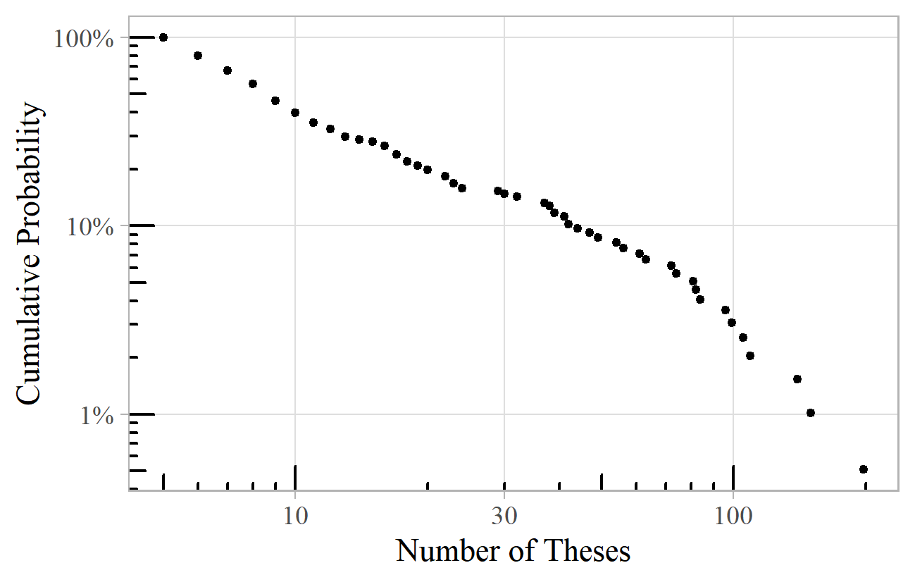
Finally, in this short survey of power laws in music history, we find them occurring in academic writing. Figure 18 shows the distribution of composers mentioned at least five times in the titles of PhD theses. 22 Composers mentioned in the titles of articles published in the Journal of the Royal Musical Association (JRMA) also follow a power law. 23 The PhD theses power law has an exponent of about 2.3, and the JRMA articles an exponent of 2.8. J. S. Bach is the top composer for PhD theses, followed by Mozart and Beethoven. Mozart is top among JRMA articles, followed by J. S. Bach and Beethoven.
HOW ARE POWER LAWS GENERATED?
All of these examples are indicators of success in the music world. Success can mean different things depending on the context – fame, sales, productivity, desirability, depth of interest, etc. The datasets are equally indicators of obscurity, a characteristic which, by sheer weight of numbers, has played a huge but largely unrecognized role in the history of music.
These distributions of musical success could easily have been quite varied. They could have followed a bell-shaped normal distribution, or had longer or shorter tails, or two or more peaks. Indeed, there is no particular reason for empirical distributions of real-world data to comply with a neat mathematical formula. So, it is remarkable not only that power laws (and the related lognormal distributions) appear so frequently in these datasets, but that they often have exponents close to two. This may indicate common processes or deeper principles governing the patterns of success and obscurity across many different musical contexts.
Power laws have been found and studied across a wide range of disciplines and contexts. Clauset, Shalizi, & Newman (2009) list many examples, including the frequency of common words; the number of connections between internet servers, or links between web pages; the intensity of wars, terrorist attacks, wildfires, solar flares, electricity blackouts, and earthquakes; the sales of bestselling books; the population of cities; the frequencies of surnames; the wealth of individuals; and the number of citations of academic papers. There are plenty of other examples in the literature. The diversity of this list indicates that many different processes can generate power laws. It is not generally possible to infer, from the existence of a power law, that a particular process is responsible for creating it.
Power laws are often produced by processes exhibiting positive feedback. Feedback is the way that the state of a process at a point in time influences its subsequent development. Negative feedback leads to extreme values tending to be followed by less extreme ones, resulting in a bounded, stable system. With positive feedback, however, extreme values tend to increase the chance of even more extreme states in the future. This is sometimes described as "the rich get richer" or as the "Matthew effect" after the following Biblical quote (Matthew 25:29, New International Version):
"For whoever has will be given more, and they will have an abundance. Whoever does not have, even what they have will be taken from them."
We see the "Matthew effect" operating with fame and popularity. Well-known people (or songs, books, ideas, etc.) often become more celebrated, simply because they are already famous. Lesser-known works are likely to get lost or forgotten and become more obscure over time.
Compare this to a case governed by negative feedback, such as the length of operas. A half-hour opera would be criticized as too short, and the composer's next one would probably be longer. Similarly, a work lasting twelve hours would be regarded as too long, and few composers would be tempted to follow suit. Thus, there is pressure for operas to cluster into a natural range of perhaps one to four hours, with an average length (say 2½ hours) being representative of a "typical" opera. There is no pressure for the length of operas to keep increasing indefinitely, and the difference between the longest and shortest operas is a ratio of perhaps three or four – much less than the factors of hundreds or thousands in some of the examples above.
To illustrate the processes that might be behind the power laws we see in musical success, here are six simple models, each generating a power law with an exponent of two.
MODEL A (SONG LISTENERS)
- There are 1,000 listeners and 1,000 songs
- In the first week, each listener listens to a random song
- In subsequent weeks, each listener…
- with 5% probability, listens to a song chosen completely at random, or
- with 95% probability, selects another listener at random, and listens to the song that that listener listened to the previous week
- After 20+ weeks, the weekly number of listeners per song is distributed roughly as a power law with exponent of about 2.0.
MODEL B (MUSIC APPRECIATION CLUB)
- A music appreciation club starts with one member and one song, the member's favorite.
- Each week, a new member joins the club, and a new song is added to the record collection. The new member…
- with 15% probability, selects a song from the club's collection to be her favorite, or
- with 85% probability, selects another member at random, and adopts their favorite song
- Members never change their favorite songs
- After 50+ weeks, the number of members favoring each song follows a power law with exponent of about 2.0.
MODEL C (CONCERT PROMOTER)
- A concert promoter organizes monthly concerts, each consisting of four works.
- She has a list of 1,000 available works.
- In the first month she selects four works at random.
- After each concert, she puts four slips of paper, containing the names of that month's works, into a bag.
- In subsequent months, she selects each of the four works as follows…
- with 10% probability, the work is selected at random from the list
- with 90% probability, the work is that written on a random slip drawn from the bag (and replaced)
- After 10+ years, the total number of times each work has been performed approximately follows a power law with exponent 2.0.
MODEL D (RANDOM WALK)
- A sheet music retailer sells publications of 1,000 works.
- In month 1, each work sells one copy.
- Subsequently, each work's sales, compared to the previous month, change by either –55%, 0%, or +55%, with each option being equally likely (sales are rounded to the nearest whole number of copies)
- A work's sales never fall below one copy per month. Or, equivalently, any work whose sales fall to zero is immediately replaced by a new work, which sells one copy in its first month.
- After 20+ months, the monthly sales by publication settles into a power law with an exponent of about 2.0.
MODEL E (EXPONENTIAL GROWTH)
- In the beginning was one musical work, which sold one copy in its first year.
- Each year, new works are created at an average rate of 10% of the total number of works existing at the start of the year. All new works sell one copy in their first year.
- The sales of each work increase by, on average, 10% per annum.
- After 100 years, the distribution of annual sales per work follows a power law with exponent of about 2.0.
MODEL F (CIRCLE OF FRIENDS)
- There are 100 people and 1,000 songs
- Everybody initially picks a list of eight songs at random
- Each person has twelve friends. These friendships were formed by everybody sitting in a large circle and getting to know the six nearest people on each side
- Friends regularly talk to each other (one to one) about the songs on their lists
- Each week, everybody selects one of their recent conversations, in which the song they spoke about was not on the list of the friend to whom they were talking. On their list, they exchange that song for…
- with one-in-eight probability, a song completely at random,
- otherwise, the song mentioned by a friend in a random recent conversation.
- Each week, the five individuals with the fewest songs in common with their friends drift away from their friendship groups and end up swapping groups randomly among themselves
- After a couple of years, the number of people having each song on their lists follows an approximate power law with exponent of about 2.0.
These models, whilst containing an element of realism, are deliberately over-simplified, designed to illustrate some ways in which power laws can arise from simple processes. The parameters (such as the probabilities of various courses of action) have been selected to produce an exponent of about 2.0 in computer simulations: changing the parameters results in a different exponent (although most reasonable values produce exponents in the range 1.5 to 3). 24 The models work just as well if songs are swapped for composers, if we exchange concerts for purchases of records or sheet music, or if time is stretched or compressed from weeks to years or days. One can conceive of more complex processes incorporating features from several of these simple models: these will also often result in power-law-like distributions. 25
Positive feedback operates in all these models. In Model A, the number of listeners of a song one week directly affects the chance of more listeners picking it the following week – so successful songs are more likely to be chosen again. Model B is similar: a song has a greater chance of being selected by a new member if it is already the selection of many existing members. The same happens in Model F, except that the pressure to swap to a new song depends on the number of friends who also like that song. In Model C, the more a work is performed, the more slips are added to the promoter's bag, and the more likely it is to be drawn again. In Model E, the positive feedback simply comes from time – the oldest works have been there longest, and everything grows at the same rate. Model D's positive feedback is more subtle: the monthly increase or decrease in sales is symmetric apart from the constraint that sales never fall below one. The positive feedback, in effect, comes from the random walk reflecting off this minimum value.
All these factors come into play in the real world. Music increases in popularity the more it is heard, or the more people have bought it or talked about it. Works that have previously been programmed at a concert may be seen as lower risk by promoters as there is known to be an audience familiar with them. Time is also important: many of us prefer to listen to old music rather than take a chance on something completely new. And the subtle process at work in Model D is not unlike the popular music charts where a record dropping out of the top 100 is immediately replaced.
Unfettered positive feedback would result in an ever-narrowing focus on a few popular works, and it is the element of randomness that limits this and leads to the diverse spectrum from popularity to obscurity that often follows a power law. Models A, B, C, and F all have small probabilities of new works being introduced into the system. This also happens in the real world. Popular music has an established process by which new music is produced, identified, promoted, and given its chance of fame. Classical concerts often include a contemporary work alongside better-known pieces. In all genres, fans will happily explore new or unfamiliar works by composers or performers that they already know. Users of online music providers are likely to be presented with new suggestions, based on the recommendations or listening habits of others.
Model F, via the shuffling of friendship groups among those with fewest songs in common, includes some randomization of the model itself. This provides some extra mixing: without it, two or three songs can dominate different segments of the circle of friends, truncating the power law at the top end. In the real world, of course, music is a powerful source of social bonding, interaction and identity, and there are almost certainly strong links between social networks and the power-law popularity of music in different styles and genres. 26
Several of these models require knowledge of the market. In Model A, each listener must know which songs the other listeners were enjoying the previous week. The popular music record charts would perhaps provide similar information in the real world. In Model C, the concert promoter creates her own list of previous data, which forms a key part of the selection procedure. In Model B, the exchange of information could happen as new recruits talk to existing members, a process made more explicit in Model F. In the real world there are many mechanisms for disseminating information on the market: critics, reviews, recommendations, awards, charts, advertising, social media, and others.
In some models there is a growing population (Model B and, by implication, Model E): others have a fixed number of people. There may be a limited number of musical works (Models A, C, D, and F), or a growing number. In practice, the quantities of music are continually increasing, and audiences grow older, die off, and are replaced by new members (as do composers and performers). Versions of these, and other, models might operate simultaneously at multiple scales across various groups of people, different styles of music, and a range of media and formats. It is perhaps impossible to model in detail, but it is nevertheless conceivable that all these interlocking processes might lead to the sort of power-law-like behavior seen in the examples above. 27
Although the six models all generate similar power law distributions of musical success, they work very differently, and this is reflected in the ways in which individual works become successful or fall into obscurity. In Model E, for example, age is the main factor defining success, and the first work inevitably becomes, and remains, the most popular. A similar thing occurs in Models B and C, where the early works have an advantage, which they retain.
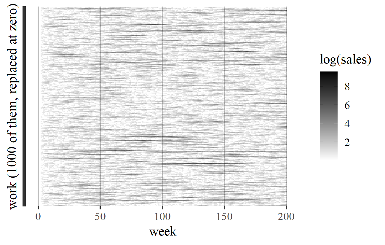
In Model D, in contrast, success is transient: works remain successful only for as long as they enjoy a run of positive or zero growth. This is like getting a run of heads in successive tosses of a coin: such runs do happen, but they rarely last long. A successful work's luck will soon run out, and another will replace it at the top of the chart. This is illustrated in Figure 19, which shows a simulation of Model D. The works (or their replacements if they fall to zero) are shown as horizontal lines, with time running from left to right. The darkness of the lines is proportional to the logarithm of the works' sales. In fact, every work (or its replacement) in Model D is destined to be the top-selling work at some point.
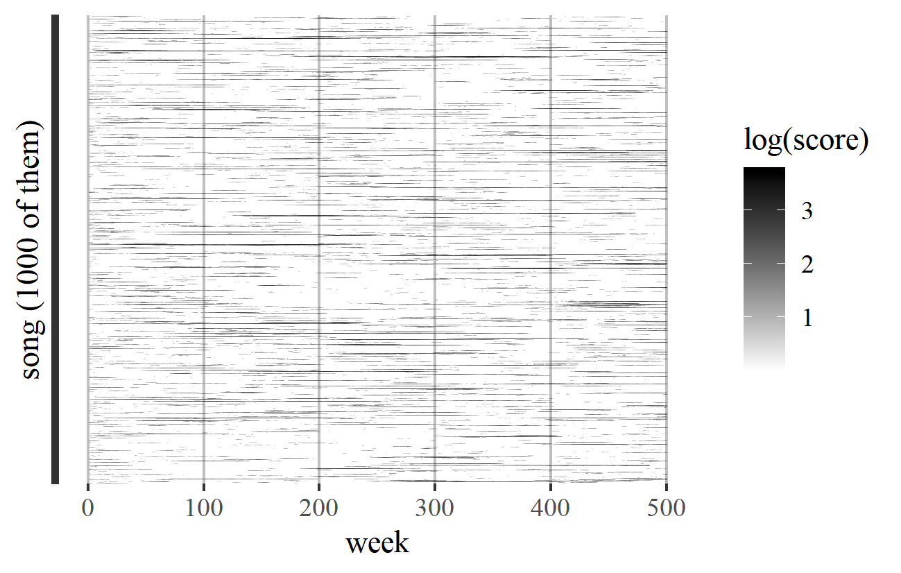
Between the stability of Models B, C, and E, and the volatility of Model D, Models A and F are more balanced. Figure 20 shows a typical transience pattern for Model F, where a few songs spend long (but still limited) periods at the top, and others never win any significant popularity at all.
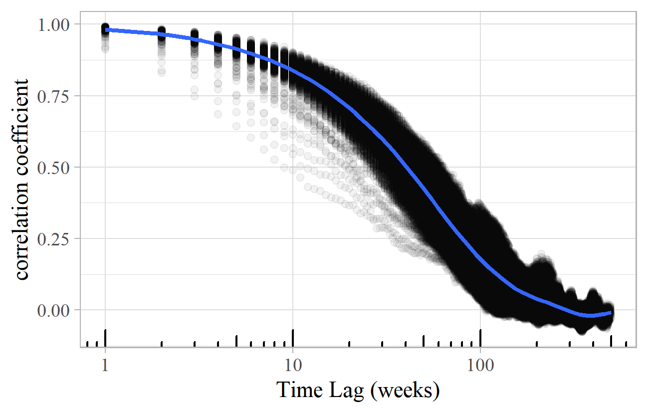
Whilst there is clearly a qualitative difference between these transience plots, they are hard to interpret and compare. A more objective way of quantifying these transience patterns is to calculate the correlation between the success scores at different times. This involves taking two points in time, and calculating the correlation coefficient between the success scores of all songs at those times. 28 These values, for all combinations of times, can be plotted on a chart such as Figure 21, which shows the lagged correlation coefficients for a typical simulation of Model F. Each point on the chart shows a pair of weeks, according to the difference between them (on the horizontal axis – note the logarithmic scale), with the correlation between the popularity of the songs at those two points indicated on the vertical axis. There is high correlation (almost 100%) between the popularity in successive weeks (i.e., lag 1) on the left of the chart, and it takes about 40 weeks for the correlation to fall to 50%. There is practically no correlation between the levels of popularity at times separated by 200 weeks or more.
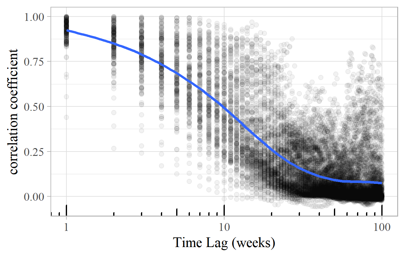
For Model D, the lagged correlation chart is shown in Figure 22. The one-week correlation is again close to 100%, and the average falls to 50% after about 12 weeks, and to zero after around 50. The most noticeable difference compared to Model F is the wide range of correlation for each value of the time lag – the period between 10 and 30 weeks includes correlations covering almost the full range from zero to one, whereas in Model F they are closely clustered around the trend line.
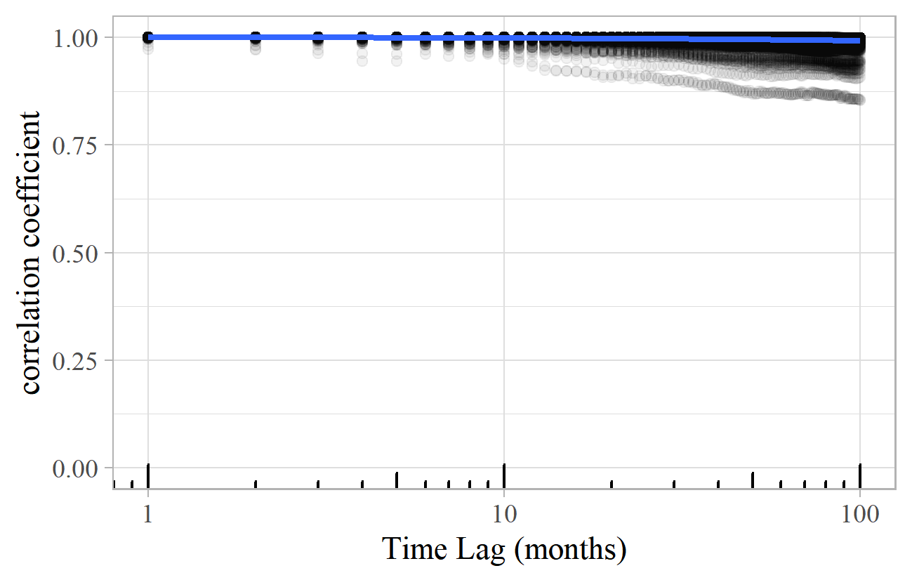
For models with low transience, the picture is rather different. Figure 23 shows the lagged correlation plot for Model C. The correlation is high for all time lags. The first works become the most popular and stay at the top indefinitely.
The lagged correlation chart is therefore a characteristic fingerprint of the dynamic processes going on in each model, even though they all, on the face of it, generate a similar power-law distribution.
It is interesting to compare these simple models with examples of transience in the real world. There are a few datasets that contain date-stamped information that enables an analysis of the transience of musical success. Among those mentioned above, these include the number of performances at the BBC Proms or by the New York Philharmonic and the appearance of composers in the titles of theses and journal articles. Before looking at these, I will consider another example: transience in the UK Top 100 Singles charts for the years 1990–99. 29
Although the record charts do not directly exhibit power law behavior (because they are rankings rather than actual sales volumes), they are an excellent source for analyzing the transience of success as reflected in the rates of record sales. As previously noted, several studies have concluded that power laws apply to various aspects of the popular music market, so although data on actual sales volumes is not readily available, it is likely that they follow a power law.
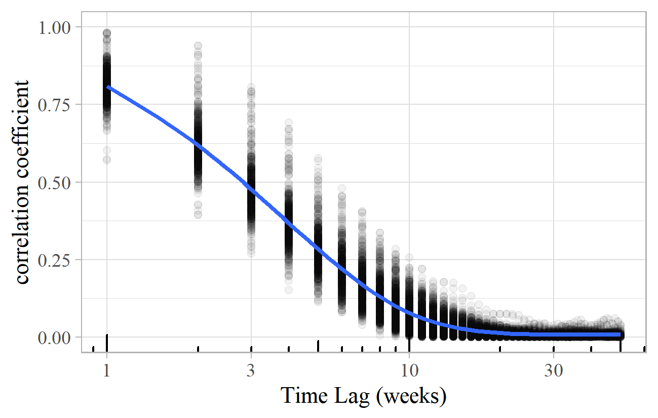
Figure 24 shows the lagged correlation plot for the weekly UK Top 100 Singles Charts for 1990-99. There is good correlation of around 80-90% from one week to the next, but this falls rapidly, reaching 50% after just three weeks, and hitting zero after about 15 weeks. The values are reasonably bunched around the trend line. (A similar, but slower decline occurs for the album charts, with 50% correlation after six weeks, and zero after about 50 weeks. The "Classical Artist" album charts are slower still, reaching 50% correlation after eleven weeks, and taking about 100 weeks to reach zero.)
What does this tell us about the processes at play in the popular music singles market? Assuming that the real market is some sort of hybrid of the models described above (and others), we might tentatively conclude that the high levels of transience suggest more Model D, with perhaps a bit of Models A and F, and relatively little of B, C, and E. A hypothetical model for popular record sales might be based on a combination of a multiplicative random walk, with elements of peer-pressure and influence from social networks (which could include broadcast music and other media).
In contrast to the singles chart, Figure 25 shows a lagged correlation plot for the number of New York Philharmonic performances of composers during each year of the twentieth century. Year-on-year correlation is high at around 75% (with quite a wide variation), and it stays at that level for a long period. 50% correlation is only reached after about 70 years.
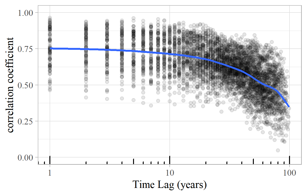
Figure 25. Lagged correlation plot for composers performed annually by the New York Philharmonic during the 20th century.
A similar pattern applies to the composers mentioned in the titles of theses and journal articles. Analyzing the number of appearances of composers in titles of PhD theses over five-year periods from 1950-2014, for example, yields the lagged correlation plot shown in Figure 26. Again, there is about 75% correlation for long periods (with a wide range), only reaching 50% on average after 35 years.
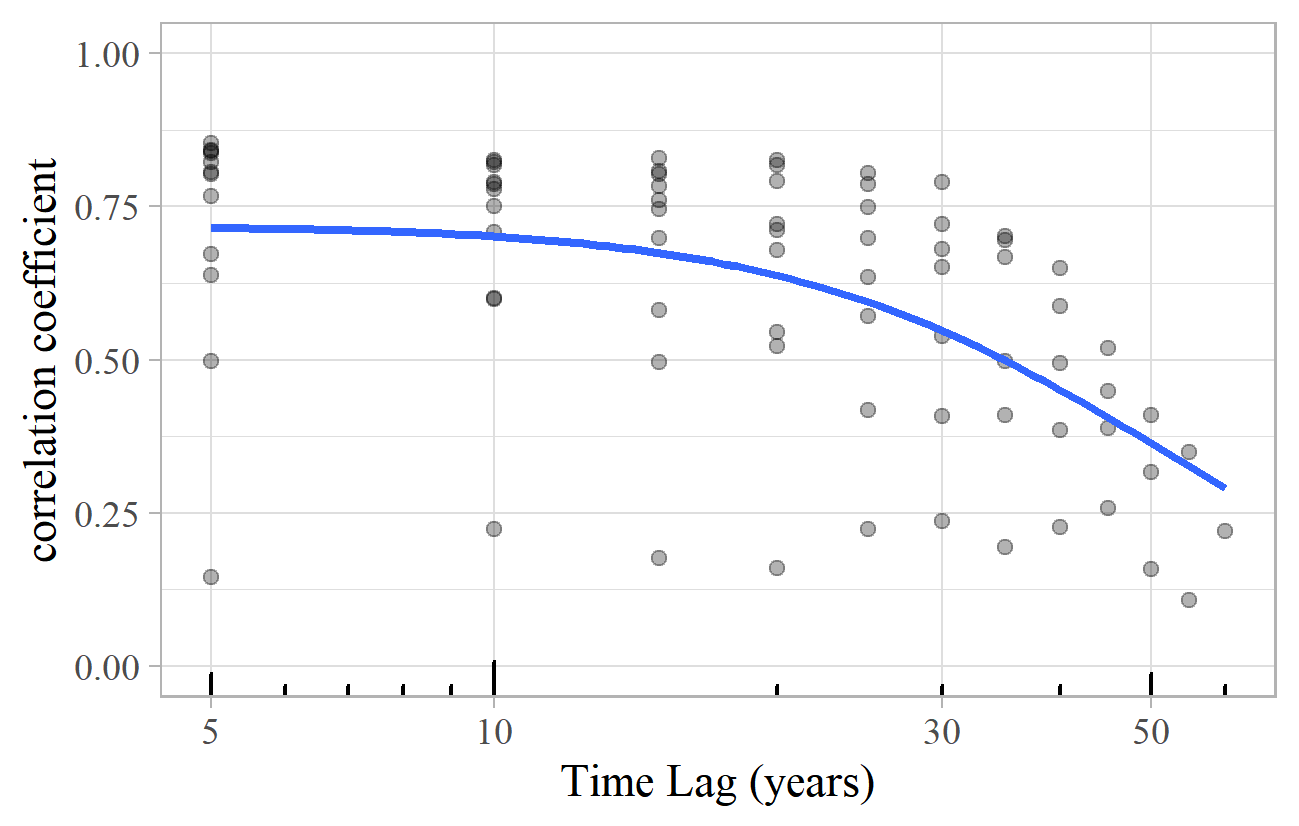
Figure 26. Lagged correlation plot of composers in PhD thesis titles in five-year periods from 1950-2014.
These classical music examples are clearly governed by different processes from that operating in the popular music singles chart. The models determining success in classical music performances and scholarly activity are perhaps more like the low transience of Models B, C, and E, with perhaps an element of Models A and F, but no sign of the volatility of Model D. This market seems to be built on the continuation of long-term track records, on stable preferences, and on a respect for previous generations of listeners and opinion-formers (it is striking that high correlation persists well beyond the lifespan of audiences). Whilst there is room for new music, novelty, and changes of direction, displacing the established big names looks to be extremely difficult.
It is no surprise that success is governed by different processes in the popular music singles chart and among the composers of classical music – after all, the two cases differ in almost every way. Teasing out the detail for specific cases is challenging, perhaps impossible, because there are alternative measures of success in different contexts, and little available data that provides a direct comparison between, for example, classical and popular music, between record sales and live performances, or between success as a composer and success as a performer. There are complex interactions between live performances, broadcast airplays, record sales, sheet music sales, critical reception, and scholarly attention, not to mention the impact of external influences such as social networks, peer pressure, and other socio-economic and cultural factors.
WHAT ABOUT INHERENT MUSICAL QUALITY?
Conspicuous by its absence from the discussion so far is the concept of musical quality – whether pieces of music are inherently "good" or "poor". In the simple models described above, all the selections and choices are made at random – either directly or by copying previous random choices. None requires any aesthetic preferences, nor an assessment of the quality of individual works. The power laws that we see in musical success can be generated without having to invoke a concept of quality: it is quite possible for these patterns to appear entirely through the operation of chance.
It is straightforward to build an allowance for quality into these models, for example by giving "good" works a higher probability of being selected than "poor" ones. They still produce power laws, often with a similar exponent. However, models that allow for quality tend to display lower transience than those that do not. Figure 27 shows a lagged correlation plot for Model F, with and without a quality effect. The songs' inherent quality was incorporated by assigning numbers from 1 to 1,000 to the songs and using these numbers to weight each song's probability of being selected, either from the songs mentioned by friends (on the basis that they are more likely to talk about the better songs) or randomly. Both versions of the model produce a power-law distribution with an exponent of 2.0, but the one allowing for quality has higher correlation at all time lags, as the better songs tend to rise to the top and stay there for longer. Without a quality effect the correlation reduces to 50% after 40–50 weeks, but with quality, it takes over twice as long and does not quite reach zero within the 500 weeks of this simulation.
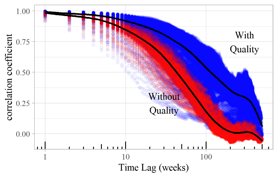
Figure 27. Lagged correlation plot of simulations of Model F both with (blue) and without (red) an allowance for inherent work quality.
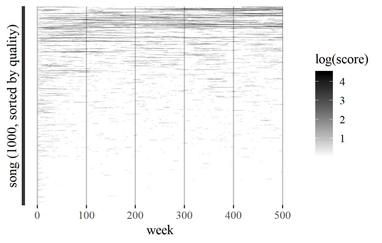
A work's inherent quality is no guarantee of success. Figure 28 is a transience plot for Model F allowing for quality, where the works (on the vertical axis) are ordered by quality, with the best at the top. As expected, quality seems to be associated with success (although the correlation coefficient between the quality and success scores is only about 35%). Several songs of middling quality enjoy runs of modest success; and near the top there are works moving in and out of favor, a few with no obvious success at all, and the most successful works (with the darkest lines) often a little below the "best". 30
The slower decay of correlation in the "quality" version of Model F perhaps lends some support to the argument that there is an inherent quality attribute affecting long-term correlation in the success of classical composers. The rapid decay of correlation in the popular music singles charts (Figure 24) might suggest that there is less of a quality effect in that market. However, it would be wrong to leap too readily to these conclusions. The impact of quality on the models generating power-law distributions is subtle and hard to distinguish from what happens purely on the basis of chance. Inherent quality is difficult to quantify, and it may, or may not, affect music choices and preferences in many ways. 31 Even if a convincing model could be constructed, there is little available data to enable it to be calibrated or directly compared with real world examples.
Among classical composers, there are both similarities and differences across the datasets representing different perspectives. The same big names will tend to appear towards the top of the list whether one considers concert performances, record sales, sheet music sales, biographical articles or academic writing. On the other hand, the order often differs: we have seen Wagner, Beethoven, Bach, and Mozart at the top in different contexts, for example. What we have not considered is how success in the concert hall influences success in record sales or academic writing, or vice versa. There is almost certainly an effect, but it would be hard to quantify. More significantly, it is likely that such interactions would mutually support each other, leading to greater stability in the patterns of success, thus having a similar effect on transience as that of inherent quality. This potentially undermines the evidence that there is, indeed, anything other than randomness at work.
Nevertheless, it is not unreasonable to suppose that our musical choices and preferences are influenced by some sort of inherent quality attribute, whatever the style, genre, or means of consumption. Influenced, but not determined: we can all recognize the imperfect correlation between quality and success and can cite (but rarely agree on) terrible pieces of music that are very successful and wonderful works that are unjustly neglected. Musical preferences and perceived quality are clearly determined in different ways depending on the context. They might be related to critical or commercial success, to reputation (among friends or knowledgeable commentators), to technical skill or sophistication, or to originality and innovation. Quality might reside in forms that persist through the generations (as in classical music), or it might express a reaction against established values or aesthetics (as in some popular music). This is a big subject and a diversion that is rather beyond the scope of this paper.
FAMILIARITY, NOVELTY AND MAXIMUM ENTROPY
This line of argument does, however, suggest another way of thinking about the origins of power laws in musical success. Perhaps the patterns of fame and obscurity and the debates and disagreements about what constitutes musical quality result from the tension between the opposing forces of familiarity and novelty. Several of the models above involve copying the choices of others or repeating what has been done before (familiarity), but also include the possibility of encountering something completely new (novelty). The power laws seem to emerge from the struggle to find a balance between these extremes. I can recognize this tension at an individual level: much as I enjoy and admire the works of Bach, The Beatles, and Miles Davis, my record collection also includes music by Sigfrid Karg-Elert, Pete Atkin, and Sahib Shihab. The first three names (and their music) are familiar to many people, and they generate wide admiration, interest, and discussion. They are an important part of our cultural fabric and play a social role in bringing people together. The latter three names, though, are relatively unknown. They do not generate any great level of record sales, scholarly attention, or debate. They are, however, important to me (all the more so because of the fact that you, the reader, probably have not heard of them!) The tension between the familiar and the novel can thus also be seen as that between the socially shared and the personal. The successful and obscure ends of the music spectrum perform different functions, both of which are important in different contexts.
Why might this tension result in a power law? A simple answer is that we have already seen several cases where this tension exists (explicitly or implicitly), and the result is a power law. There is, however, a more fundamental argument that can explain power laws as a consequence of the "law of maximum entropy". This is an important and widely applicable principle that says that systems tend to progress (within the constraints of the system) towards a state of maximum disorder or minimum predictability. The principle is important in the physical sciences, biology, computing, and information theory, and increasingly in applications in the social sciences and humanities such as economics, linguistics, and the movement of people within and between cities (Hernando, Hernando, Plastino, & Plastino, 2012).
A familiar example of the law of maximum entropy is that the molecules of gas in a closed box will, at any moment, tend to be distributed evenly throughout the box. A uniform distribution of gas molecules is the solution, subject to the constraints that everything must stay inside the box and obey the normal laws of physics, that maximizes the disorder or entropy (a mathematical way of quantifying disorder). This does not say anything about the process by which this solution occurs. It is, in a sense, a purely statistical result that formalizes the observation that things tend to get more messy, disordered, and unpredictable over time. A similar argument could be applied to people in a room, socks in a drawer, or fish in a pool: the underlying processes and interactions would obviously be different, but the end result – maximum disorder and an even distribution – would be the same.
A power law is also the solution to a maximum entropy problem but with a different constraint: that the average of the logarithm of the value is equal to a fixed number. The "value" here is our measure of musical success – record sales, appearances at the BBC Proms, etc. – and the "fixed number" is directly related to the exponent of the power law. For a continuous power law with exponent a, the mean of the logarithm of the variable is equal to 1/(a–1) (using "natural" logarithms). For a power law exponent of two, the average of the natural logarithm of the success measure would be equal to one. Derivation of the power law as the solution to this maximum entropy problem is given by Visser (2013).
If we regard the power laws of musical success as a consequence of the law of maximum entropy, there are two important corollaries. The first is that there is indeed a more universal principle at work, which helps to explain why power laws appear so often in different contexts, despite being produced by quite different processes. The mechanisms by which power laws are formed – including our six models – are just alternative ways in which the maximum entropy principle takes effect. They are processes that allow disorder to increase in the right sort of way, within the constraints of the system. It takes a more detailed examination of the dynamics of the system (such as with a lagged-correlation analysis) to tell the models apart – the power law itself is not enough.
The second insight relates to the constraint that the average of log(musical success) should be constant. The implication is that it is not the direct measures of musical success that are most meaningful (record sales, concert appearances, etc.) but rather their logarithms. Logarithms convert multiplication to addition so measures of success should be compared by their ratios, not their differences. So, if composer A has 5,000 concert appearances and composer B has 2,500, we can say that the difference between A and B is the same, in a sense, as that between composers C and D, where C has 20 appearances and D has 10. If composer E had 4,990 appearances, we would not feel comfortable concluding that the gap between A and E was the same as that between C and D, even though the difference is 10 in each case. Intuitively this feels right: musical success does seem to be a multiplicative characteristic, so its logarithm is additive. The constraint that produces a power law is simply that this log-success score should have a particular average value.
Let us return to the number of appearances of composers at the BBC Proms. The number of times a composer's works have been performed ranges from one (44% of composers) to 6,100 (Wagner). We now know that a more meaningful measure of success is the logarithm of these values – so the single-appearance composers score zero (=log(1)), and Wagner would score 8.7 (=log(6100)). 32 The distribution of composers by the logarithm of the number of appearances is as follows (Table 1):
| log- appearances | Appearances | Number of composers | Proportion of composers | Proportion of appearances |
|---|---|---|---|---|
| 0 – 1 | 1 – 2 | 1,460 | 59% | 3.1% |
| 1 – 2 | 3 – 7 | 530 | 21% | 3.8% |
| 2 – 3 | 8 – 20 | 236 | 9.5% | 5.0% |
| 3 – 4 | 21 – 54 | 122 | 4.9% | 6.9% |
| 4 – 5 | 55 – 148 | 76 | 3.0% | 11.6% |
| 5 – 6 | 149 – 403 | 36 | 1.5% | 15.7% |
| 6 – 7 | 404 – 1096 | 20 | 0.80% | 21.6% |
| 7 – 8 | 1097 – 2980 | 7 | 0.28% | 21.7% |
| 8 – 9 | 2981 – 8103 | 1 | 0.040% | 10.5% |
The log-appearance values increase linearly, representing an ever-widening range of the number of appearances, as shown by the second column. The number of composers in each range decreases – roughly halving each time as we move down the table. The average value of log-appearances comes out at 1.1, heavily weighted by the majority of composers falling into the first 0–1 band. This is the value we expect from the fact that the power law exponent is around 1.9 (i.e., 1/(1.9–1)).
We can subjectively test the reasonableness of a logarithmic success scale by selecting names corresponding to regularly-spaced values of the logarithm of the number of appearances and judging whether the perceived gaps between successive names seem to be about equal. Taking values from the BBC Proms data with log-appearances approximately equal to 8, 7, 6, 5, 4, 3, 2 gives the sequence Beethoven – Elgar – Schumann – Parry – Poulenc – Léhar – Cherubini, which, bearing in mind the British context, does not seem unreasonable. Another sequence, using the New York Philharmonic data and log-scores of 8½, 7½, 6½,… 2½, would be Tchaikovsky – Dvořák – Bizet – Schoenberg – Kabalevsky – C. P. E. Bach – Milton Babbitt.
The success scales depend on the size of the dataset. If there had only been ten years of BBC Proms concerts, for example, Wagner might still be at the top, but he would have a lower log-success score (of perhaps 5–6). Most of the top names would be similar, but many of the obscure composers would probably not appear at all. The average would still be about 1.1. We could do the same analysis with any of the previous examples and would get the same pattern – a logarithmic success scale, rapidly decreasing numbers as the scale increases, and an average log-success score close to 1/(exponent–1).
Some of the earlier log-log plots were a little too curved to be confidently labeled as power laws, and it was noted that they might be better described by a lognormal distribution. The lognormal is also the solution to a maximum entropy problem where the constraint is a fixed average log-success score. In this case, there is an additional constraint: that the log-success should also have a fixed spread (or variance) about its mean value. Some of the examples that deviate most noticeably from the straight line of a power law are those where there is likely to be human intervention in the editing or compilation of the data – the selections chosen for the Penguin Record Guides or the length of articles in biographical dictionaries. It seems that, left alone, the music market will produce power-law-like distributions, but when there is human involvement in curating the data, there is also some management of the relative spread. Obscure composers or works are less likely to be included, and the really big names might be pared back so as not to seem excessive.
The final column of Table 1 shows the proportion of BBC Proms performances accounted for by the composers in each group. These figures increase as the log-success score rises (apart from the last one, but this only has one member). Over half of BBC Proms performances are accounted for by the 28 composers in the three highest groups, and the 59% of composers with just one or two appearances only account for just over 3% of performances. This helps to explain why the average value of log-appearances feels like a rather low 1.1 – it is an average over composers, most of whom are quite obscure. In practice, concert promoters and audiences are probably more interested in how much time is allocated to the different groups, so an average weighted by the total level of activity would arguably make more sense.
If the probability that a random composer has x appearances is proportional to 1/xa (i.e., a power law with exponent a), then the probability that a random performance is by a composer with x appearances is proportional to this value weighted by x, i.e., x/xa, or 1/xa-1, which is just another power law with exponent a-1. If one of these power laws is being created by the law of maximum entropy, then so is the other – they are just alternative expressions of the same thing.
This observation provides a clue as to why musical success power laws tend to have an exponent of about two. If these power laws have exponents close to two, then the derived ones, weighted by the levels of activity, must have exponents of about one. The usual formula for the average log-success of a power law breaks down if the exponent equals one, as 1/(exponent-1) = 1/(1-1) = 1/0, which is infinite and therefore problematic. In practice, real data is always finite, and the trick is to set a maximum value M based on practical considerations for the topic at hand. It can then be shown that, to get an exponent exactly equal to one, the power law is the solution to the maximum entropy problem subject to the constraint that the mean of the log-success is ½log(M) (Visser, 2013, pp. 7-8). In terms of Table 1, this is saying that the average log-success band (weighted by activity) should be the middle one.
Actually, for the BBC Proms data, the average log-success band weighted by activity is above the middle value, because the proportions in the final column of Table 1 increase as the log-success rises. This is because the exponent of the BBC Proms power law, 1.9, is less than two. If it had been higher than two, we would have found the proportions in the final column decreasing as the log-success increased, so that the activity from the big-name composers was less dominant. For an exponent of exactly two, the proportions in the final column would stay roughly constant from one log-success band to the next (although the highest and lowest bands are likely to deviate from this rule).
Figure 29 uses simulated power laws with various exponents to show the proportion of total activity in each log-success band, calculated in the same way as for the last column of Table 1. Exponents in the range 1.9–2.1 are reasonably level across the bands, so each band contributes about the same amount of activity. Exponents of 1.7 or 2.3 show noticeable increases or decreases, and exponents of 1.5 or 2.5 are more extreme, with quite significant variation between the lowest and highest bands.
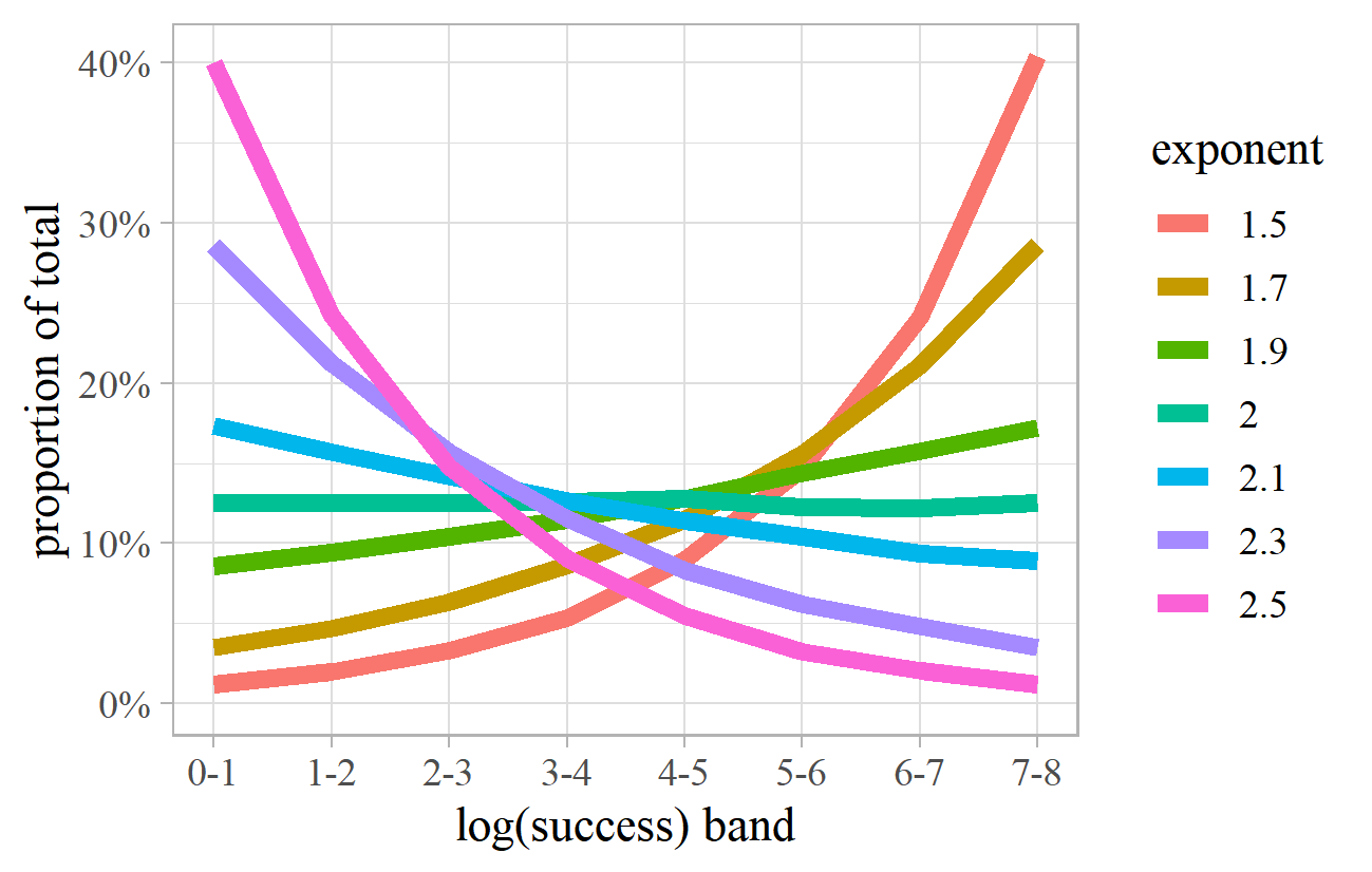
Figure 29. Proportion of total activity by log-success band for simulated power laws with various exponents.
So, our maximum entropy argument equates to the constraint that the log-success, when weighted by the total activity, is evenly distributed across the range of the data. This is what causes the exponent of the activity-weighted power law to be close to one, and that of the success score itself to be about two. This "principle of evenly distributed log-success" is analogous to the law that leads to an even distribution of gas molecules in a closed box. Our natural measure of musical fame and obscurity, log-success, spreads itself evenly so that the total amount of activity is roughly constant across the range between zero and its maximum value. Like gas molecules, this is a dynamic system, constantly changing but always retaining a roughly even spread. The rate of change is analogous to the temperature of the gas: hot for the rapid changes in popular music record sales, cool for the slow shifts of fortune among classical composers.
The simple models in this paper all had their structure and parameters selected to produce a power law with an exponent of two. They would all have worked perfectly well with different parameters, so the choice was, in that sense, arbitrary. However, we now see that there is a deeper principle at play: whatever the process generating the power law behavior of musical success in the real world, the principle of evenly distributed log-success will cause its parameters to be pushed in a direction that leads to an exponent close to two. Table 2 summarizes the previous examples, sorted by exponent:
| Example | Exponent | Comments |
|---|---|---|
| Fétis 1837 Pages per Composer | 1.8 | Probably lognormal |
| New York Philharmonic Composers | 1.8 | |
| VW Memorial Library Folk Songs | 1.8 | Significant curvature |
| Pazdírek Works per Composer | 1.8 | |
| BBC Proms Composers | 1.9 | |
| Penguin Guide 1988 Recordings per Work | 1.9 | |
| Penguin Guide 1999 Recordings per Work | 1.9 | |
| Penguin Guide 2007 Recordings per Work | 1.9 | |
| Songs per Artist in MLDB | 2.0 | High curvature suggests lognormal |
| Gerber 1812 Pages per Composer | 2.0 | Possibly lognormal |
| Number of Cover Versions of Songs | 2.0 | |
| New York Philharmonic Works | 2.1 | |
| Proms Haydn Symphonies | 2.2 | |
| Number of Recordings per Opera Singer | 2.2 | Significant curvature |
| British Library Publications per Composer | 2.2 | |
| IMSLP Works per Female Composer | 2.2 | |
| Penguin Guide 1975 Recordings per Work | 2.3 | |
| Eitner 1900 Pages per Composer | 2.3 | Possibly lognormal |
| Mendel 1870 Pages per Composer | 2.3 | |
| Composers in PhD Thesis Titles | 2.3 | |
| IMSLP Sampled Appearances of Composers | 2.4 | |
| Oxford Music Online Composer Article Lengths | 2.5 | Clearly lognormal |
| Composers in JRMA Article Titles | 2.8 | Relatively small dataset |
| BBC Proms Works | 2.9 | Bend in line at about 70 performances |
| Top 1000 Rare Record Prices - Classical | 3.3 | |
| Top 1000 Rare Record Prices - Rock | 3.4 | |
| Top 1000 Rare Record Prices - all genres | 3.4 | |
| Top 1000 Rare Record Prices - Jazz | 4.2 | More curved than other genres |
| UK Top 60 Album Sales | 4.8 | Only the extreme tail of distribution |
| UK Million-selling Singles | 4.9 | Only the extreme tail of distribution |
The warning about the difficulty of accurately estimating the exponents of empirical power laws should be borne in mind. Nevertheless, we observe a high degree of clustering in the range 1.8-2.5. The exponent for Composers in JRMA Journal Titles at 2.8 is rather high although it is quite a small dataset, so we should expect a higher margin of error in the estimate. It might also indicate something about the criteria by which articles are accepted for publication, perhaps to give greater prominence to lesser names. The BBC Proms Works exponent of 2.9 also stands out as a little high, which could be at least partly due to an apparent bend in the straight-line at around 70 performances (see Figure 4). Estimating the exponent based on the average slope of the line (rather than using the usual "maximum likelihood" estimate) comes out at about 2.4.
Several of these examples show a slight downward curvature on a log-log plot, rather than the perfect straight line of an exact power law. This will, other things being equal, tend to give slightly greater weight to the activity of the higher log-success bands. In these cases, an estimated exponent a little higher than two will offset this curvature to produce a more even distribution across the bands.
The examples that do not appear to fit our theory are rare record prices and the top selling albums and singles. These are based only on the extreme tails of the distributions so do not necessarily reflect prices or sales overall. They might, for example, simply be the ends of otherwise lognormal distributions. Comprehensive data on record sales is impossible to find in the public domain, and I know of no studies that have investigated the distribution of the entire market.
Record prices are a fundamentally different measure of success from the other examples. All of the others are based on counts (of sales, works, words, recordings, etc.), but prices are qualitatively different: a monetary agreement between a buyer and a seller, reflecting their perceptions of value, scarcity, and desirability. The argument about activity-weighted power laws does not translate directly to measures of success based on prices. It is beyond the scope of this paper to pursue this argument further, but there may well be a line of argument linking these price-based power laws (if indeed they are power laws) to principles and processes similar to those for count-based ones.
Despite these exceptions, the fact that many empirical power laws have exponents close to two suggests that market forces conspire to ensure that each log-success band of works, composers, or performers makes a similar contribution to the overall level of activity. This is a manifestation of balancing the tension between the popular, familiar, culturally and socially important music at the top end of the scale and the novel, eclectic expressions of individuality at the other.
CONCLUSIONS
We have seen that many measures of success in the history of music are approximately distributed according to a power law, often with an exponent close to two. We have explored several simple models which can produce such power laws. Examining their lagged-correlation fingerprints suggests parallels with some of the historical music examples, giving clues to the ways that success and obscurity emerge in those contexts and shedding some light, albeit dimly, on the existence or otherwise of inherent musical quality. We then argued that these models are all manifestations of a more fundamental process resulting from the Law of Maximum Entropy, subject to the constraint that the average of the logarithm of the success scores is constant. This in turn implied that success is a multiplicative quality (with log-success as its natural measure), and that musical markets operate to strike a balance between familiarity (socio-cultural importance) and novelty (individual importance). The exponent of about two emerges as a result of the "principle of evenly distributed log-success", a tendency for musical activity to be spread evenly across the log-success bands.
This explanation is coherent and evidence-based but is inevitably approximate. These are empirical distributions that appear to be power laws, but some are clearly more power-law-like than others. The mathematics has been simplified, partly because many other authors have developed this in detail, partly to present an understandable narrative to non-mathematicians, and partly because with such real-world historical data, the most we can hope for is that theory is a rough reflection of messy reality. Whilst there is plenty of data on the success and obscurity of musical works, composers, performers, and recordings, it is simply the data that happens to exist rather than what we would ideally want in order to study success in a scientific way. There are complex interactions between the participants in the musical world; between the variety of forms that music can take; between genres, regions, and periods; and with numerous external cultural and socio-economic factors. There are further complications associated with musical quality and aesthetics and with the relationship between different measures of success (live performances, broadcasts, record sales, publications, academic reputation, etc.). Even if we could build a model incorporating all these things, we would not have the data to calibrate it, and there would be too many moving parts to understand what was going on.
Several of the datasets here are probably better described by a lognormal distribution rather than a power law (although it is not always easy to tell the difference, and there is no particular reason why this data should follow a simple mathematical formula at all). The line of argument has been pursued principally for power laws (as it is simpler), but it would be interesting to extend the analysis to investigate the circumstances better described by a lognormal distribution.
Much has been written about power laws in many fields in the physical and human sciences, as becomes quickly evident on examining the bibliographies of some of the references cited in this article. Many authors have developed in detail the mathematics of power laws, including several variants of the simple form we have encountered here. There are numerous examples of empirical power laws, and much discussion of the ways in which power laws can be generated. Having read a lot of this literature whilst preparing this paper, it occurs to me that two useful and important ideas have not been adopted as widely as I would expect. The first is the observation that a power law weighted by activity is just another power law with the exponent reduced by one. This can significantly shift the perspective of a problem. In this paper, it was the key step in the argument leading to the principle of evenly distributed log-success, enabling an explanation of why the exponents of these observed power laws tend to be roughly equal to two. 33
The second neglected idea is that of power laws as dynamic, rather than static (or simply growing), systems. Success in the music world is a process that evolves through time, and this is reflected in the simple models discussed in the paper as well as the processes that take place in the real world. An observed power law in a dataset may often be simply an accumulation or snapshot of a richly dynamic and evolving process. To really understand what is going on, we need to think about, and if possible, measure, how the system evolves. This can give important indicators of the processes and parameters by which power laws are created.
It is remarkable that, across a wide range of genres, context and methods of experiencing music, we – audiences, record buyers, scholars, concert programmers – unwittingly conspire to allocate fame and obscurity to musical works, composers and performers in such a way that the same patterns of success arise again and again. The process is one of enormous complexity, yet behind it lie some simple principles that ensure that we enjoy an optimum balance in which our collective attention is evenly distributed across the spectrum between the big names that form an important part of the fabric of our culture and society and the little-known ones that ensure an endless supply of new and unfamiliar music.
ACKNOWLEDGEMENTS
This article was copyedited by Niels Chr. Hansen and layout edited by Diana Kayser.
NOTES
-
Correspondence can be addressed to Andrew Gustar by email at andrew@gustar.org.uk. Further work on this topic may be published on my website https://www.musichistorystats.com.
Return to Text -
See https://www.bbc.co.uk/proms/archive.
Return to Text -
The data was collected with a computer program that worked through each concert page and collected the relevant details. All of the analysis for this paper has been carried out using the statistical programming language R (R Core Team, 2019), and the charts have been produced using ggplot2 (Wickham, 2016).
Return to Text -
The key feature of logarithms is that they convert multiplication into addition: so the logarithm (or, commonly, just the "log") of 2 times 100, is the log of 2 plus the log of 100.
Return to Text -
Raising to the power a means multiplying a number by itself a times. So 2 raised to the power 3, written 23, is equal to 2*2*2=8. If a is not a positive whole number, this is less intuitive, but it can be well-defined mathematically. If x = ab, then log(x) = b * log(a).
Return to Text -
A power law shows as a straight line on a log-log plot whether you draw x against p(x), or against the cumulative probability (i.e., the probability of being at least x, rather than exactly equal to x). All the power law charts in this paper are log-log plots using the cumulative probability. Some mathematical details of power laws have been simplified or ignored in this paper – such as failing to distinguish between the discrete and continuous cases. This does not affect the overall reasoning. Power laws are sometimes referred to, in different contexts and subject areas, as Zipf, Lotka or Pareto distributions.
Return to Text -
See https://archives.nyphil.org/index.php/open-data.
Return to Text -
Estimating the exponents of power laws – especially approximate empirical ones – is not straightforward. I give estimates to one decimal place, but the "true" value may be slightly different. I have used the maximum likelihood estimator as described by Clauset, Shalizi, and Newman (2009).
Return to Text -
Sources differ on the number of Haydn symphonies. For simplicity, I will assume that there are 104.
Return to Text -
See https://www.bl.uk/bibliographic/download.html#basicmusic.
Return to Text -
See https://www.vwml.org.
Return to Text -
See https://imslp.org/.
Return to Text -
These were based on random samples of 100 works from each guide. See Gustar (2014), 40-41.
Return to Text -
The data is from Wikipedia: https://en.wikipedia.org/wiki/List_of_best-selling_albums_in_the_United_Kingdom.
Return to Text -
The vertical axis on Figure 11 shows "Rank" rather than the cumulative probability. As the data only covers the top 60 albums, it is impossible to tell the proportion of the total market accounted for by these titles. Cumulative Probability = Rank / Total Number of Items, so the two only differ by a constant factor, and using Rank will therefore still produce a straight line on a log-log plot.
Return to Text -
See http://www.mldb.org/.
Return to Text -
See https://secondhandsongs.com.
Return to Text -
See http://www.valueyourmusic.com.
Return to Text -
The data is from https://www.operadis-opera-discography.org.uk/.
Return to Text -
The data originate from Gustar (2014, pp. 41–43), using Gerber (1812), Fétis (1837), Mendel (1870), and Eitner (1900).
Return to Text -
See https://www.oxfordmusiconline.com.
Return to Text -
As listed by the American Musicological Society at https://www.ams-net.org/ddm/.
Return to Text -
See https://www.tandfonline.com/loi/rrma20.
Return to Text -
There are many sources describing processes that generate power laws, which have been used to create these models. A couple of examples are Mitzenmacher (2004) and Simkin and Roychowdhury (2011).
Return to Text -
This appears to be the case with more complex models that I have played with although it is difficult to prove more generally. It can be shown, for example, that combinations of power laws (or other "heavy-tailed" distributions) result in power laws. See, for example, Willinger, Alderson, Doyle, & Li, 2004).
Return to Text -
Power laws commonly arise in the structure of social and other networks, and it is possible that these directly influence the development of power laws in music success. For a review of power laws in networks, see Keller (2005).
Return to Text -
Models A, B, C, and F all have "zero-success" works that are not chosen, played or listened to. Although in the discussion above it appeared to be possible to estimate the total number of Haydn symphonies by extrapolating from those that had been performed at the BBC Proms, there is no evidence, from carrying out the same procedure on these models, that this approach works in general.
Return to Text -
The correlation coefficient measures the extent to which high values of one variable correspond to high values of another. A correlation coefficient of +1 indicates a strong tendency to move in line with each other. A coefficient of –1 means that high values in one set correspond to low values in the other. A coefficient of zero suggests that there is no particular linear relationship between the two sets of values.
Return to Text -
This period was selected somewhat arbitrarily, but with the intention of avoiding the complications associated with digital music downloads and streaming. All data is from the Official Charts Company at https://www.officialcharts.com.
Return to Text -
To some extent this pattern is due to how quality has been assigned. The top 10% of works, for example, only vary in quality score between 900 and 1000, affecting their probabilities of being selected by no more than 10%. Another approach would produce a different pattern. I do not know of any research quantifying the quality of musical works, so this remains a difficult question to pursue further.
Return to Text -
Studies have shown that "following the crowd" has a significant impact on musical success, irrespective of objective quality. A particularly interesting study, for example, is the "Musiclab" experiment, where listeners selected music both with and without knowledge of the broader popularity of the tracks. See Salganik, Dodds, and Watts (2006) and Salganik and Watts (2008, 2009).
Return to Text -
This value is the natural logarithm of 6,100, which on many calculators and spreadsheets is called ln rather than log. You might also find logarithms to base 10, for which the value of log10(6100) is about 3.8. The natural logarithm is always about 2.3 times larger than the log to base 10. It does not matter which one you use, as long as you are consistent. All of the logs in this paper are natural logarithms.
Return to Text -
There are relatively few theoretical explanations in the literature of why empirical power laws have the exponents they do. One example, deriving the exponent of one often observed in the power laws describing the distribution of city sizes, is Chen (2011).
Return to Text
REFERENCES
- Chen, Y. (2011). The rank-size scaling law and entropy-maximizing principle. Physica A, 391((3), 767–778. https://doi.org/10.1016/j.physa.2011.07.010
- Clauset, A., Shalizi, C. R., & Newman, M. E. J. (2009). Power-law distributions in empirical data. SIAM Review, 51(4), 661–703. https://doi.org/10.1137/070710111
- Cox, R. A. K., Felton, J. & Chung, K. H. (1995). The concentration of commercial success in popular music: an analysis of the distribution of gold records. Journal of Cultural Economics, 19(4), 333–340. https://doi.org/10.1007/BF01073995
- Eitner, R. (1900). Biographisch-bibliographisches Quellen-Lexikon der Musiker und Musikgelehrten christlicher Zeitrechnung bis Mitte des neunzehnten Jahrhunderts. Leipzig, Germany: Breitkopf & Haertel.
- Fétis, F.-J. (1837). Biographie universelle des musiciens et bibliographie générale de la musique. Paris, France: Firmin-Didot.
- Gerber, E. L. (1812). Neues historisch-biographisches Lexikon der Tonkünstler. Leipzig, Germany: A. Kühnel.
- Greenfield, E., Layton, R. & March, I. (1975). The Penguin Stereo Record Guide. London, UK: Penguin.
- Greenfield, E., Layton, R. & March, I. (1988). The New Penguin Guide to Compact Discs and Cassettes. London, UK: Penguin.
- Greenfield, E., Layton, R. & March, I. (1999). The Penguin Guide to Compact Discs. London, UK: Penguin.
- Gustar, A. J. (2014). Statistics in historical musicology. PhD thesis, Open University, UK. Retrieved from http://oro.open.ac.uk/41851/
- Haampland, O. (2017). Power laws and market shares: cumulative advantage and the billboard hot 100. Journal of New Music Research, 46(4), 356–380. https://doi.org/10.1080/09298215.2017.1358285
- Hernando, A., Hernando, R., Plastino, A., & Plastino, A. R. (2012). The workings of the maximum entropy principle in collective human behaviour. Journal of The Royal Society Interface, 10(78). https://doi.org/10.1098/rsif.2012.0758
- Keller, E. F. (2005). Revisiting "scale-free" networks. BioEssays, 27(10), 1060–1068. https://doi.org/10.1002/bies.20294
- Keuchenius, A. (2015). The evolution of a new music genre as an expanding network: a quantitative systems approach to study innovation in the creative economy. M2 Project Report, University of Warwick, UK. Retrieved from https://warwick.ac.uk/fac/cross_fac/complexity/study/emmcs/outcomes/studentprojects/m2_project_anna_keuchenius.pdf
- Koch, N. M. & Soto, I. M. (2016). Let the music be your master: power laws and music listening habits. Musicae Scientiae, 20(2), 193–206. https://doi.org/10.1177/1029864915619000
- Krueger, A. B. (2019). Rockonomics. London, UK: John Murray.
- March, I, Greenfield, E., Layton, R., Czajkowski, P. (2007). The Penguin Guide to Recorded Classical Music. London, UK: Penguin.
- Mendel, H. (1870). Musikalisches Conversations-Lexikon: Eine Encycklopädie der gesammten musikalischen Wissenschaften (H. Mendel, Ed.). Leipzig, Germany: Verlag von Robert Oppenheim.
- Mitzenmacher, M. (2004). A brief history of generative models for power law and lognormal distributions. Internet Mathematics, 1(2), 226–251.https://doi.org/10.1080/15427951.2004.10129088
- Pazdírek, F. (Ed.) (1904-1910). The universal handbook of musical literature: practical and complete guide to all musical publications. Vienna, Austria: Pazdírek & Co.
- R Core Team. (2019). R: A language and environment for statistical computing. Vienna, Austria: R Foundation for Statistical Computing. Retrieved from https://www.R-project.org/
- Salganik, M. J., Dodds, P. S. & Watts, D. J. (2006). Experimental study of inequality and unpredictability in an artificial cultural market. Science, 311(5762), 854–856. https://doi.org/10.1126/science.1121066
- Salganik, M. J. & Watts, D. J. (2008). Leading the herd astray: an experimental study of self-fulfilling prophecies in an artificial cultural market. Social Psychology Quarterly, 71(4), 338–355. https://doi.org/10.1177/019027250807100404
- Salganik, M. J. & Watts, D. J. (2009). Web-based experiments for the study of collective social dynamics in cultural markets. Topics in Cognitive Science, 1(3), 439–468. https://doi.org/10.1111/j.1756-8765.2009.01030.x
- Simkin, M. V. & Roychowdhury, V. P. (2011). Re-inventing Willis. Physics Reports, 502(1), 1–35. https://doi.org/10.1016/j.physrep.2010.12.004
- Visser, M. (2013). Zipf's law, power laws, and maximum entropy. New Journal of Physics, 15(4), [XXX]. https://doi.org/10.1088/1367-2630/15/4/043021
- Wickham, H. (2016). ggplot2: elegant graphics for data analysis. New York, NY: Springer-Verlag. https://doi.org/10.1007/978-3-319-24277-4
- Willinger, W., Alderson, D., Doyle, J. C. & Li, L. (2004). More "normal" than normal: scaling distributions and complex systems. In R. G.Ingalls, M. D. Rossetti, J. S. Smith, & B. A. Peters (Eds), Proceedings of the 2004 Winter Simulation Conference (pp. 130–141). Hanover, MD: Institute for Operations Research and the Management Sciences. https://doi.org/10.1109/wsc.2004.1371310

