
Introduction
THE nPVI ("normalized pairwise variability index") equation quantifies the average difference between adjacent events in a sequence (musical notes in a melody, successive vowels in a spoken sentence). While originally developed by phoneticians to classify language based on their rhythmic differences, more recent work has shown this statistic can be used to quantify musical rhythm and uncover historically relevant musical changes over time (Daniele and Patel, 2004; Daniele and Patel, 2013; Daniele and Patel, 2015; Hannon, 2009; Hannon et al., 2016; Hansen et al., 2016; McGowan and Levitt, 2011; Patel and Daniele, 2003; Patel et al., 2006; Temperley and Temperley, 2011; VanHandel and Song, 2010). Building upon an earlier finding that German/Austrian composer mean nPVI values increased steadily from 1600 to 1950 (while Italian composers showed no such increase), the nPVI distribution of themes was quantitatively explored. 2 In Daniele 2016 I reported the proportion of "low" nPVI or "Italianate" themes decreased steadily with time while "high" nPVI (more Germanic) themes increased in frequency. "Middle" range nPVIs exhibited a constant incidence and so I argued for a replacement of "low" nPVIs (Italianate) with "high" nPVIs (Germanic) over a short time instead of a modest, long-term progressive shift (the "Replacement Hypothesis"). A survey of the musicological record identified the rise in musical nationalism in Germany/Austria from 1760 to 1800 could be influencing this trend (Daniele, 2016; Morrow, 1997). VanHandel's assessment of the data, however, highlighted an alternate hypothesis which notes that the rise of the "New German School" and "Wagnerians" (composers who identified with Richard Wagner over the more traditional "Brahmsian" style) after 1825 could affect the observed rise in "high" nPVI frequencies (VanHandel, 2016). Upon reanalysis, this paper finds similar results to the original Daniele 2016 article but highlights that VanHandel's historical assessment is most likely correct and proposes a new tool, the "rhythmic fingerprint," to enable future research to better quantify and classify rhythmic influence than a single value representation (e.g. composer mean nPVI) could.
Methods
Theme List, Exclusion Criteria, and Data Analysis
Data was collected, computed, and analyzed according to the previous methods and exclusion criteria enumerated extensively in Daniele & Patel 2013. As in the Daniele & Patel studies, the musical materials for the current work were drawn from A Dictionary of Musical Themes, Revised Edition (Barlow and Morgenstern, 1983). Seventy-five (75) musical themes was the cutoff for generating an nPVI frequency plot for an individual composer while fifteen (15) themes was the cutoff for calculating a composer's mean nPVI. The midpoint year (the mathematical average of the birth and death year, representing when the composer was active, abbreviated "ca.") was used to plot composers over time. A k-means clustering test, an unbiased grouping algorithm, was used to classify composers into two categories (k = 2) based on their "midpoint year" and "mean nPVI". A k-means test clustered all composers with a midpoint year before 1790 as "Baroque/Classical Era" (1600-1750/1750-1810) while those after 1790 were considered the "Romantic Era" (1825-1900) and this fits closely with the musicological record (Kmetz et al., 2001). Notably, the k-means test reliably classified Beethoven as a Romantic composer despite him writing most of his compositions during the "Classical period" (Indy, 1970; Solomon, 1998). For frequency plots, the nPVIs of individual themes were grouped based on their values e.g. nPVI = 0-5, 5-10, 10-15, to 140+, and the number of themes within each range was tallied. When plotting the data, the frequency values were then plotted as a percentage (%) of the total themes of that composer (y) vs. the nPVI range (x).
Results
Similar Findings after a Reanalysis of Daniele 2016
One criticism of the original Daniele 2016 manuscript was that Baroque and Classical composers were underrepresented and "Wagnerian" composers from the Romantic era were overrepresented which, together, could cause nPVI values to trend upward in the late 1800's. To decrease this potential bias, ten composers were added to the corpus and new medians were calculated for grouped "Baroque/Classical" composers (nPVI = 32.2, Table 1, Yellow) and "Romantic" composers (nPVI = 39.2, Table 1, Blue). 3 These values were used to demarcate "low" (nPVI < 32.2), "middle" (nPVI > 32.2 and < 39.2), and "high" (nPVI > 39.2) tiers for each composer's theme corpus (Table 1). It should be noted that the intercept point of the German/Austrian and Italian regressions was an nPVI = 41.3 (Daniele and Patel, 2013) which makes an nPVI of 39.2 a reasonable demarcation point for moving away from the "Italian" style.
| Composer | # themes | Midpoint Year | Median nPVI | Mean nPVI | % themes w/ nPVI < 32.2 | % themes w/ 32.2<nPVI<39.2 | % themes w/ nPVI>39.2 |
|---|---|---|---|---|---|---|---|
| Buxtehude | 16 | 1672 | 22.6 | 29.0 | 68.8 | 12.5 | 18.8 |
| J.S. Bach | 351 | 1717.5 | 24.9 | 27.5 | 65.8 | 12.0 | 22.2 |
| Telemann | 32 | 1724 | 34.4 | 37.9 | 43.8 | 18.8 | 37.5 |
| C.P.E. Bach | 17 | 1751 | 38.3 | 43.8 | 35.3 | 17.6 | 47.1 |
| Haydn | 278 | 1770.5 | 33.3 | 35.8 | 48.9 | 11.5 | 39.6 |
| Mozart | 460 | 1773.5 | 38.9 | 41.7 | 39.1 | 11.3 | 49.6 |
| Beethoven | 487 | 1798.5 | 38.1 | 43.0 | 40.5 | 11.1 | 48.5 |
| von Weber | 48 | 1806 | 39.9 | 45.1 | 37.5 | 12.5 | 50.0 |
| Schubert | 232 | 1812.5 | 42.8 | 47.1 | 28.0 | 13.8 | 58.2 |
| Mendelssohn | 145 | 1828 | 36.1 | 39.9 | 43.4 | 11.7 | 44.8 |
| Schumann | 216 | 1833 | 37.9 | 41.2 | 42.1 | 8.3 | 49.5 |
| Wagner | 82 | 1848 | 63.6 | 63.9 | 46.3 | 6.1 | 74.4 |
| Suppé | 30 | 1857 | 48.5 | 52.8 | 26.7 | 10.0 | 63.3 |
| Bruckner | 60 | 1860 | 49.4 | 48.8 | 20.0 | 15.0 | 65.0 |
| J.Strauss, Jr. | 95 | 1862 | 57.1 | 55.1 | 19.5 | 16.8 | 62.1 |
| Brahms | 362 | 1865 | 41.1 | 43.5 | 34.5 | 10.8 | 54.7 |
| Bruch | 15 | 1879 | 52.0 | 58.0 | 20.0 | 6.7 | 73.3 |
| Mahler | 57 | 1888.5 | 45.0 | 46.0 | 21.1 | 21.1 | 57.9 |
| Reger | 23 | 1894.5 | 40.0 | 41.3 | 47.8 | 0.0 | 52.2 |
| R. Strauss | 111 | 1906.5 | 59.0 | 60.0 | 39.0 | 10.8 | 72.1 |
| Hindemith | 65 | 1929 | 46.3 | 49.0 | 23.1 | 7.7 | 69.2 |
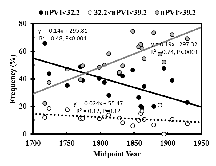
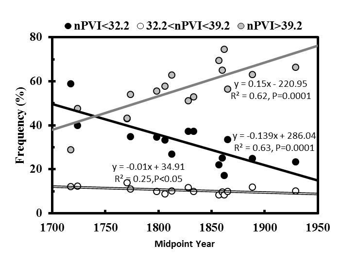
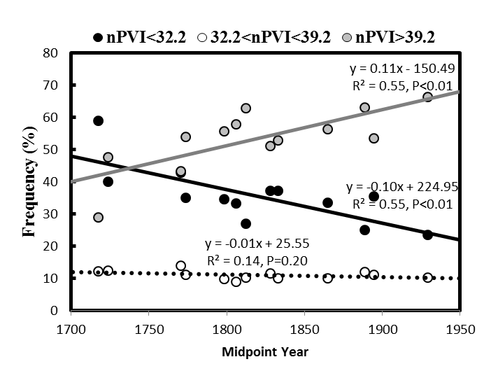
When nPVI frequencies for "low", "middle", and "high" tiers were plotted against midpoint year the regressions for "low" nPVI (<32.2) and "high" nPVI (>39.2) frequencies were very significant (Figure S1A). Notably, regressions for "high" and "low" nPVI frequency tiers vs. midpoint year were still significant when "New German School" composer data (Wagner, Suppé, Bruckner, J. Strauss, Jr., Bruch, and R. Strauss) was excluded (Figure S1B). Further, this phenomena does not appear to be dependent on the presence of composer data after the ~1825 divide of German music into the "Brahmsian" and "New German" schools (analysis included Mendelssohn, "low" nPVI frequency regression, R2 = 0.44, P<0.01, and "high" nPVI tier regression, R2 = 0.70, P<0.001, data not shown). As in Daniele 2016, the "middle" tier nPVI frequency vs. midpoint year regressions were not significant in any of these plots. By comparison, a similar analysis on Italian composers (Table 2) found no significant regressions for any nPVI tier when plotted against midpoint year (Figure S2).
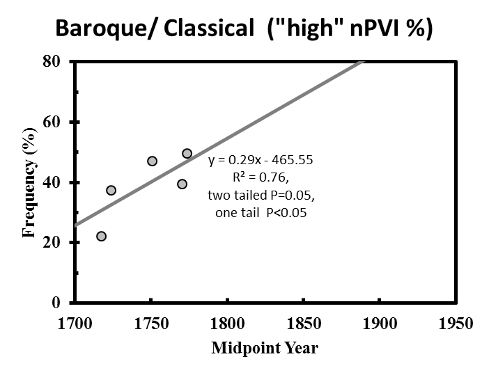
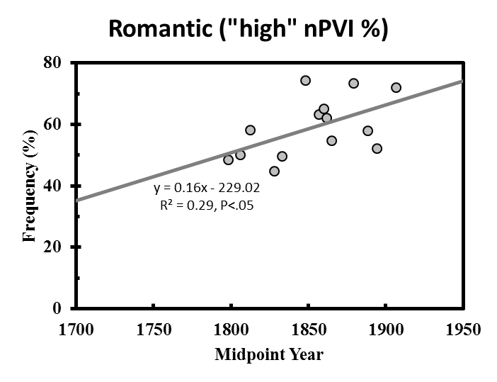
I have shown that (1) a significant upward trend in the frequency of "high" nPVI themes can be observed in nPVI data preceding the rise of "Wagnerian" composers and (2) that this trend is not observed in Italian music. But what if "high nPVI" frequencies vs. "midpoint year" from solely Baroque/Classical and solely Romantic composers are plotted (as in VanHandel 2016, Figure S3A and S3B)? My reanalysis found that the frequency of "high" nPVI themes from Baroque/Classical composers and Romantic composers also rises with time (Figure S3A and S3B). This suggests that both data sets have a tendency to trend upward in nPVI with respect to midpoint year.
Finally, using my updated composer list, I tested how nPVI frequency varies under conditions when nPVI increased incrementally with time using a computer simulation from Daniele 2016 (Figure S4A-B). 4 Previously, and in this manuscript with a revised composer list, I found that "middle" nPVI frequency decreases significantly in simulation but did not observe this in the actual composer data (compare to Figure S1). Thus, I concluded that "low" nPVI themes were quickly and dramatically being replaced with "high" nPVI themes around the late 1700s - early 1800s (the "Replacement Hypothesis"). However, when "Wagnerian"/ "New German School" composers were excluded, the regression for "middle" range nPVI proportions vs. midpoint year was no longer significant (compare Figure S4A to S4B). This suggested that the "Wagnerians"/ "New German School" composers, which possess an unusually high frequency of "high nPVI" themes, are shaping these rising nPVI trends (hypothesized in VanHandel 2016). My findings differ slightly from VanHandel 2016 but we both come to the same conclusion; that a comprehensive understanding of historical musicology is important to tease apart patterns seen in nPVI over time.
| Composer | # themes | Midpoint Year | Median nPVI | Mean nPVI | % themes w/ nPVI < 32.2 | % themes with 32.2<nPVI<39.2 | %themes w/ nPVI>39.2 |
|---|---|---|---|---|---|---|---|
| Corelli | 30 | 1683 | 47.4 | 47.6 | 23.3 | 6.7 | 70.0 |
| Vivaldi | 50 | 1709.5 | 27.2 | 35.5 | 64.0 | 4.0 | 32.0 |
| Tartini | 22 | 1731 | 32.7 | 37.8 | 45.5 | 9.1 | 45.5 |
| Paganini | 26 | 1811 | 38.9 | 40.6 | 42.3 | 7.7 | 50.0 |
| Rossini | 24 | 1830 | 44.8 | 39.0 | 33.3 | 12.5 | 54.2 |
| Verdi | 21 | 1857 | 45.1 | 47.3 | 33.3 | 4.8 | 61.9 |
| Respighi | 47 | 1907.5 | 44.1 | 49.0 | 27.7 | 10.6 | 61.7 |
| Casella | 17 | 1915 | 29.9 | 34.1 | 52.9 | 29.4 | 17.6 |
| Malipiero | 15 | 1927.5 | 43.3 | 43.9 | 20.0 | 20.0 | 60.0 |
The "Rhythmic Fingerprint"
NPVI frequency tiers help remove bias in representing each composer as a number (e.g. mean nPVI) but ideally one should want data more akin to a "fingerprint" which provides multiple points of comparison and is not dependent on parametric testing. For this, I developed the "rhythmic fingerprint" which plots nPVI distribution and allows one to classify composers based on distributional similarity.
NPVI distribution was plotted for individual composers who had written before, during, and after the proposed German shift away from the "Italianate" style (Figure 1 and Figure 2 and see Supplementary Movie). Themes with lower (e.g. more "Italian") nPVI values decrease in frequency from Bach to Beethoven, and while higher (more "German/Austrian") nPVIs increase in occurrence.
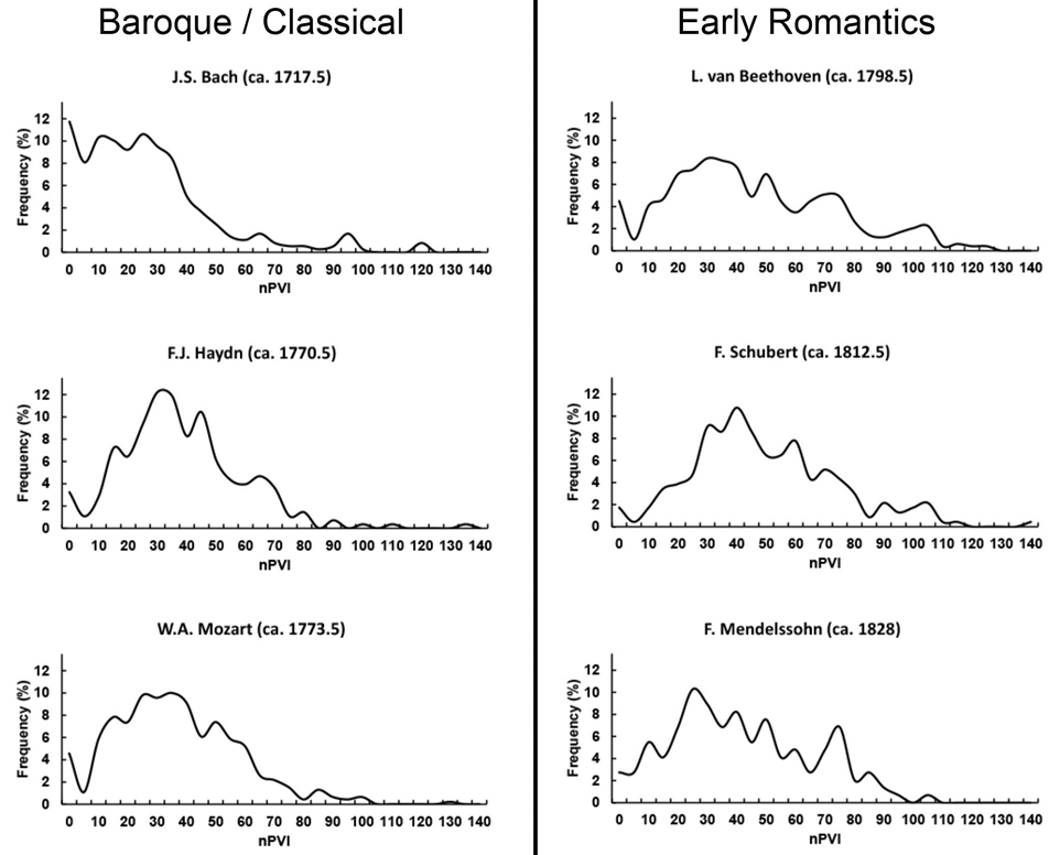
Fig. 1. Distribution of nPVI values for German/Austrian composers writing during different periods. Distributions are from composers that wrote predominantly before, during, and after the aforementioned 1760-1800 transition in German music.
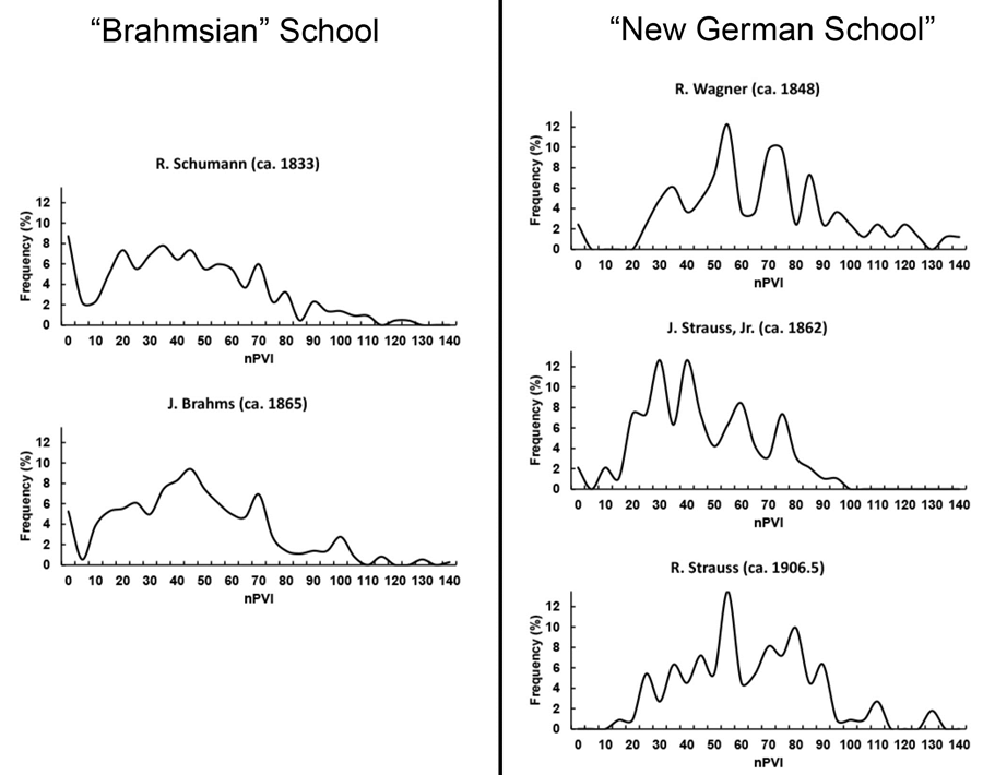
Fig. 2. Distribution of nPVI values for German/Austrian composers writing after 1825.
One can look at the shape of these distributions and see similarities as well (Figures 1 and 2). For instance, Beethoven, Schumann, and Brahms, composers of the "Brahmsian" school, have a striking similarity to one another and this can be visually represented when their rhythmic "fingerprints" are overlaid (Figure 3A). These similarities and differences are especially apparent when distributions are overlaid as in the "Brahmsian" school (Figure 3A) or the "New German" School (Figure 3B). 5
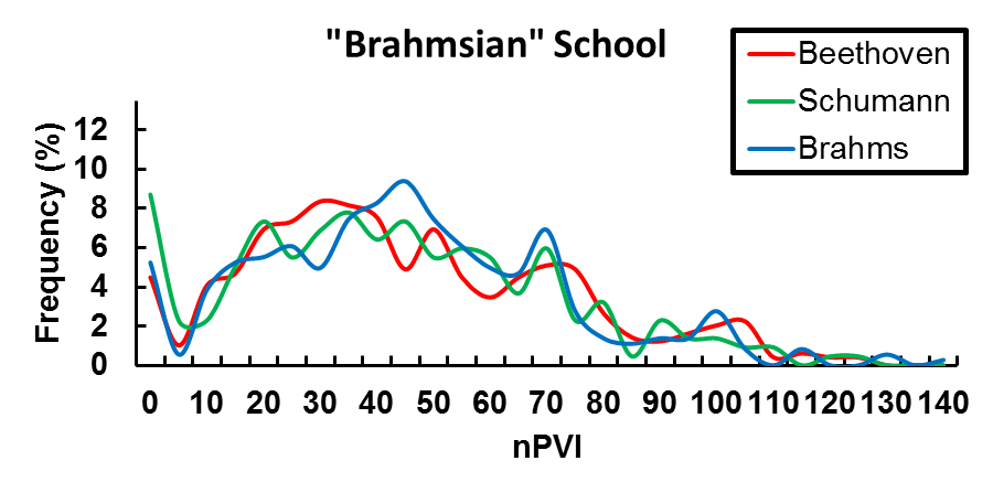
Fig. 3a. Distribution of nPVI values for "Brahmsian" School composers. Red line (Beethoven, ca. 1798.5), green line (Schumann, ca. 1833), and blue line (Brahms, ca. 1865).
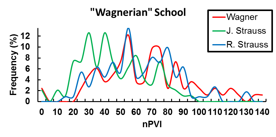
Fig. 3b. Distribution of nPVI values for "Wagnerian" School composers. Red line (R. Wagner, ca. 1848), Green line (J. Strauss, Jr., ca. 1862), and Blue line (R. Strauss, ca. 1906.5).
Notably, none of these distributions were Gaussian (Anderson-Darling Test for Normality, P<0.05) so nonparametric significance tests needed to be used. To quantitatively assess the distance between composer nPVI distributions, I applied the Kolmagrov-Smirnov (K-S) test (Table 3 & 4, statistically similar composer pairs are highlighted in YELLOW). Interestingly, no composers had a similar "fingerprint" to J.S. Bach and only Mendelssohn was similar to Haydn. Mozart, however, shared similarity with Beethoven, Mendelssohn, Schumann, and Brahms. Also, only "Wagnerian" or "New German School" composers were statistically similar to one another (Wagner, J. Strauss, Jr. and R. Strauss) (Table 4). 6
| Composer | vs. J.S. Bach | vs. Haydn | vs. Mozart | vs. Beethoven |
|---|---|---|---|---|
| J.S. Bach | D=0.24, P< 0.001 | D=0.28, P<0.001 | D=0.27, P<0.001 | |
| Haydn | D=0.24, P< 0.001 | D=0.14, P<0.01 | D=0.15, P<0.001 | |
| Mozart | D=0.28, P< 0.001 | D=0.14, P<0.01 | D=0.08, P=0.10 | |
| Beethoven | D=0.27, P<0.001 | D=0.15, P<0.001 | D=0.08, P=0.10 | |
| Schubert | D=0.39, P<0.001 | D=0.22, P<0.001 | D=0.14, P<0.01 | D=0.13, P<0.01 |
| Mendelssohn | D=0.26, P<0.001 | D =- 0.14, P=0.05 | D=0.06, P=0.73 | D=0.06, P=0.72 |
| Schumann | D=0.26, P<0.001 | D=0.16, P<0.01 | D=0.08, P=0.32 | D=0.05, P=0.90 |
| Wagner | D=0.61, P<0.001 | D=0.49, P<0.001 | D=0.39, P<0.001 | D=0.35, P<0.001 |
| Strauss, Jr. | D=0.52, P<0.001 | D=0.39, P<0.001 | D=0.28, P<0.001 | D=0.26, P<0.001 |
| Brahms | D=0.33, P<0.001 | D=0.18, P<0.001 | D=0.07, P=0.31 | D=0.08, P=0.16 |
| R. Strauss | D=0.60, P<0.001 | D=0.48, P<0.001 | D=0.37, P<0.001 | D=0.34, P<0.001 |
| Composer | vs. Mendelssohn | vs. Wagner | vs. Brahms |
|---|---|---|---|
| J.S. Bach | D=0.26, P<0.001 | D=0.61, P<0.001 | D=0.33, P<0.001 |
| Haydn | D=0.14, P=0.05 | D=0.49, P<0.001 | D=0.18, P<0.001 |
| Mozart | D=0.06, P=0.73 | D=0.39, P<0.001 | D=0.07, P=0.31 |
| Beethoven | D=0.06, P=0.72 | D=0.35, P<0.001 | D=0.08, P=0.16 |
| Schubert | D=0.18, P<0.01 | D=0.30, P<0.001 | D=0.11, P<0.05 |
| Mendelssohn | D=0.37, P<0.001 | D=0.11, P=0.18 | |
| Schumann | D=0.06, P=0.87 | D=0.36, P<0.001 | D=0.08, P=0.28 |
| Wagner | D=0.37, P<0.001 | D=0.35, P<0.001 | |
| Strauss, Jr. | D=0.29, P<0.001 | D=0.19, P=0.08 | D=0.25, P<0.001 |
| Brahms | D=0.11, P=0.18 | D=0.35, P<0.001 | |
| R. Strauss | D=0.36, P<0.001 | D=0.10, P=0.72 | D=0.32, P<0.001 |
Discussion
The present study illustrates how nPVI analysis can reveal the rhythmic underpinnings of important musical shifts and proposes a new tool to better quantify and classify rhythmic influence.
Evidence for the "Wagnerian" influence
I developed a new method to study the "metric" of a composer's style, namely the distribution and spread of nPVI for a composer's entire theme corpus. After the addition of ten composers to the corpus (to supplement with more Baroque/Classical and more non-"Wagnerian" Romantic composers) I find the same results as in Daniele 2016. I observed the frequency of themes with "low" nPVIs (< 32.2) drops dramatically with time and themes with "high" nPVIs (> 39.2) concomitantly rises with time. Themes in the "middle" nPVI range (between 32.2 and 39.2) again showed no significant trend. (Figure S1). I also observed that (1) a similar analysis of Italian composers revealed no significant linear regressions for any frequency tier (Figure S2), (2) that the proportion of "high" nPVI themes rises in isolated data sets of both Baroque/Classical and Romantic composers (Figure S3) and (3) a simulation of incremental nPVI increases with time differs significantly from the observed results though, importantly, this result depends on the presence of "Wagnerian" composers (Figure S4).
While the data without "Wagnerian" composers show significant trends (suggesting high "Germanic" nPVIs are quickly being adopted around 1760), the fact that the simulation results are indistinguishable from the observed results when "Wagnerian" composers are excluded from the analysis suggests the "Wagnerians" strongly shape these trends. This is a clear weakness of the nPVI proportion "metric" as a smaller window for "middle" range nPVIs (revised to 32.2-39.2 from 32.2-43) can make subtle trends more difficult to study.
The "Rhythmic Fingerprint"
In the process of writing this manuscript I observed that the methods in both Daniele 2016 and VanHandel 2016 were unable to distinguish major composer classes using mean nPVI or nPVI proportions alone. For instance, a k-means test could not distinguish "Brahmsian" from "Wagnerian" composers while an ANOVA could (VanHandel, 2016). However, an ANOVA failed to distinguish between "Baroque/Classical" and "Brahmsian" composers (VanHandel, 2016). Thus, I developed a new analytical tool to quantify and classify composer types based on their rhythmic distributions ("rhythmic fingerprint").
Initial analysis suggests that it wasn't until Mozart that similarities are seen between rhythmic "fingerprints" in my composer panel (Table 3). Surprisingly, Mozart's "fingerprint" is significantly different from Haydn's despite the two distributions appearing similar (D = 0.14, P < 0.01). 7 This suggests that Haydn had not yet abandoned the "Italianate" style for the "German" style but that Mozart might have been an early adopter. Musicological analysis of this time also suggests Mozart's style was considered "Germanic" (Morrow, 1997: 111, 135).
A true watershed figure in this transition, however, is Beethoven. When I compared Beethoven's nPVI distribution to that of earlier composers I observed a striking frequency shift to writing higher (more "Germanic") nPVI themes (Figure 1 & 2 and Supplementary Movie). A visual analysis of these distributions showed that composers who wrote after Beethoven had a significant proportion of "high" nPVI themes (and similar "fingerprints"). This particular "fingerprint" seems to start with Beethoven and persist through to Schubert, Mendelssohn, Schumann, and Brahms (Figures 1 & 2). A K-S test proved that these distributions were very similar (Table 3) and this is most apparent when distributions are overlaid (Figure 3A). The K-S test could also reliably identify similarities in the "Wagnerian" composers (Table 4 and Figure 3B). Notably, this test was especially useful when comparing the "fingerprint" of J. Strauss, Jr. with Beethoven since the two distributions look similar but are actually statistically quite distinct (Table 3).
An unexpected result of this analysis was the complete lack of similarity between Franz Schubert's "fingerprint" and any other composer (by K-S test). 8 This amazingly prolific composer died very young (age 32) and left 1,500+ works to his name, many of which were discovered and re-popularized after his death (Kreissle von Hellborn et al., 1869; Liszt and Suttoni, 1989). A potential line of study, for instance, could be on whether the cause of Schubert's apparently unique rhythmic style was due to the corpus used (see London, 2013) or potentially, to some other factor(s).
Finally, both these tools should enable future research with the nPVI to uncover complex stylistic trends and allow researchers to better identify and understand these shifts by quantifying their rhythmic underpinnings.
ACKNOWLEDGEMENTS
The author would like to thank Leigh VanHandel for her helpful comments during review.
NOTES
-
All correspondence should be addressed to Joseph R Daniele, Department of Molecular and Cellular Biology, University of California, Berkeley, 188 Li Ka Shing Center, Rm 430E, Berkeley, CA 94530. Email: jdaniele@berkeley.edu.
Return to Text -
This positive trend in Patel and Daniele 2013 is very robust. This regression is significant under many different conditions and combinations (e.g. using median nPVI, year when the composer age was 25, or composer birth year).
Return to Text -
This was an identical composer list to Daniele and Patel 2013. Buxtehude, Telemann, and C.P.E. Bach were now included from the Baroque/Classical era and von Weber, Suppé, Bruckner, Bruch, Mahler, Reger, and Hindemith were added from the Romantic era. Lists of grouped nPVI values from all Baroque/Classical composers or all Romantic composers were non-normal (Anderson Darling Test) so medians (instead of means) were used to bound the "low", "middle", and "high" nPVI tiers.
Return to Text -
This software assumed normal distributions to calculate nPVI proportions so only composers with 30 or more available themes were used. Normally an N≥30 data points is necessary to calculate a reliable "mean" and "standard deviation" which I deemed a prerequisite for inclusion in the simulation (Chakrapani, 2011; Kar and Ramalingam, 2013). If composer means and standard deviations from composers with N<30 themes were included in the simulation, the regressions for "low" and "high" nPVI tiers were still significant but the regression for "middle" tier nPVI frequencies was not significant (P=0.07).
Return to Text -
We did not include distribution plots with less than 75 themes. Distributions made with less than 75 themes appeared to be susceptible to over-representation in one or two bins, making the determination of their "shape" or "fingerprint" difficult to assess.
Return to Text -
A K-S test performed between R. Strauss and. J Strauss, Jr. gave a D = 0.13 and P = 0.33. There was no significant difference between the two distributions.
Return to Text -
Of note, Felix Mendelssohn's "fingerprint" was not significantly different from Josef Haydn (while all other Romantic composers were) (Table 3). This is interesting as Mendelssohn was known to derive strong influence from Baroque and Classical composers and it also suggests an important shift in rhythmic change that occurred between Haydn and Mozart's time.
Return to Text -
A K-S test performed between R. Strauss and Schubert gave D = 0.28 and P < 0.001, while Schumann vs. Schubert gave D = 0.16 and P < 0.01, and J. Strauss, Jr. vs Schubert gave D = 0.22 and P < 0.01. All other comparisons to Schubert are shown in Tables 3 and 4.
Return to Text
REFERENCES
- Barlow, H. & Morgenstern, S. (1983). A Dictionary of musical themes. London: Faber.
- Chakrapani, C. (2011). Statistical Reasoning vs. Magical Thinking: Shamanism as Statistical Knowledge: Is a Sample Size of 30 All You Need? vue 16–18. Available at: http://www.chuckchakrapani.com/articles/pdf/0411chakrapani.pdf
- Daniele, J. R. (2016). A tool for the quantitative anthropology of music: Use of the nPVI equation to analyze rhythmic variability within long-term historical patterns in music. Empirical Musicology Review, 11(2), 228–232. https://doi.org/10.18061/emr.v11i2.4893
- Daniele, J. R. & Patel, A. D. (2004). The Interplay of Linguistic and Historical Influences on Musical Rhythm in Different Cultures. In 8th International Conference on Music Perception and Cognition, 3-7.
- Daniele, J. R. & Patel, A. D. (2013). An Empirical Study of Historical Patterns in Musical Rhythm. Music Perception. 31, 10–18. https://doi.org/10.1525/mp.2013.31.1.10
- Daniele, J. R. & Patel, A. D. (2015). Stability and Change in Rhythmic Patterning Across a Composer's Lifetime. Music Perception. 33, 255–265. https://doi.org/10.1525/mp.2015.33.2.255
- Hannon, E. E. (2009). Perceiving speech rhythm in music: listeners classify instrumental songs according to language of origin. Cognition 111, 404–410. https://doi.org/10.1016/j.cognition.2009.03.003
- Hannon, E. E., Lévêque, Y., Nave, K. M. & Trehub, S. E. (2016). Exaggeration of Language-Specific Rhythms in English and French Children's Songs. Auditory Cognitive Neuroscience. 939. https://doi.org/10.3389/fpsyg.2016.00939
- Hansen, N. C., Sadakata, M. & Pearce, M. (2016). Non-linear changes in the rhythm of European art music: Quantitative support for historical musicology. Music Perception, 33(4) 414–431. https://doi.org/10.1525/mp.2016.33.4.414
- d'Indy, V. (1970). Beethoven: A Critical Biography. New York: Da Capo Press.
- Kar, S. S. and Ramalingam, A. (2013). Is 30 the magic number? issues in sample size estimation. Natl J Commun Med 4, 175–179.
- Kmetz, J., Finscher, L., Schubert, G., Schepping, W. & Bohlman, P. V. (2001). Germany. In: S. Sadie (Ed). In The New Grove Dictionary of Music and Musicians, pp. 708–744. New York: Grove.
- Kreissle von Hellborn, H., Coleridge, A. D. & Grove, G. (1869). The Life of Franz Schubert. London, Longmans, Green, and co.
- Liszt, F. & Suttoni, C. (1989). An Artist's Journey. University of Chicago Press.
- London, J. (2013). Building a Representative Corpus of Classical Music. Music Perception 31(1), 68–90. https://doi.org/10.1525/mp.2013.31.1.68
- McGowan, R. W. & Levitt, A. G. (2011). A Comparison of Rhythm in English Dialects and Music. Music Perception, 28(3), 307–314. https://doi.org/10.1525/mp.2011.28.3.307
- Morrow, M. S. (1997). German music criticism in the late eighteenth century: aesthetic issues in instrumental music. Cambridge, U.K.; New York: Cambridge University Press. https://doi.org/10.1017/CBO9780511549427
- Patel, A. D. & Daniele, J. R. (2003). An empirical comparison of rhythm in language and music. Cognition 87, B35–B45. https://doi.org/10.1016/S0010-0277(02)00187-7
- Patel, A. D., Iversen, J. R. & Rosenberg, J. C. (2006). Comparing the rhythm and melody of speech and music: the case of British English and French. J. Acoust. Soc. Am. 119, 3034–3047. https://doi.org/10.1121/1.2179657
- Solomon, M. (1998). Beethoven. New York; London: Schirmer Books; Prentice Hall International.
- Temperley, N. & Temperley, D. (2011). Music-Language Correlations and the "Scotch Snap." Music Percept. Interdiscip. J. 29, 51–63. https://doi.org/10.1525/mp.2011.29.1.51
- VanHandel, L. (2016). The War of the Romantics: An Alternate Hypothesis Using nPVI for the Quantitative Anthropology of Music. Empirical Musicology Review, 11(2), 234–242. https://doi.org/10.18061/emr.v11i2.5474
- VanHandel, L. & Song, T. (2010). The Role of Meter in Compositional Style in 19th Century French and German Art Song. J. New Music Res. 39, 1–11. https://doi.org/10.1080/09298211003642498
Appendices
Appendix A
S1A: All German/Austrian Composers
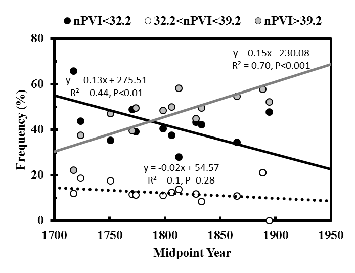
S1B: "New German School"/ "Wagnerian" Composers Excluded
Fig. S1. Percent of themes within a particular range for each German/Austrian composer plotted against midpoint year (see Table 1). Three vertical dots (black, grey, and white), representing the percent of themes within a particular nPVI range for each composer are plotted against composer midpoint year. Linear regressions were computed from the proportion of themes, for each composer, within an nPVI range. Lines represent significant linear regressions (P<0.01). Dotted lines represent non-significant linear regressions. Minimum number of themes per composer = 15. Figure S1A displays all composer nPVI tier frequencies while Figure S1B has excluded "New German School" and "Wagnerian" composers.
Appendix B
S2: All Italian Composers
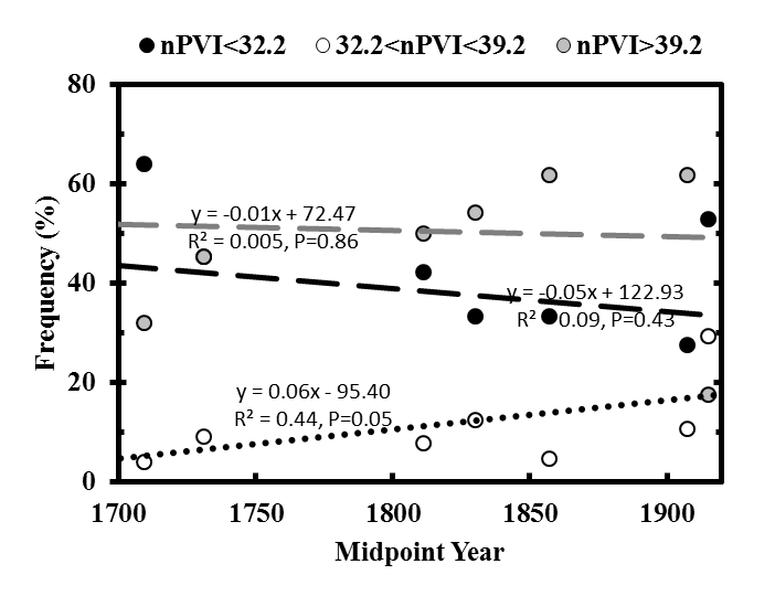
Fig. S2. Percent of themes within a particular range for each Italian composer plotted against midpoint year (see Table 2). Three vertical dots (black, grey, and white), representing the percent of themes within a particular nPVI range for each composer are plotted against midpoint year. Linear regressions were computed from the proportion of themes, for each composer, within an nPVI range. Dotted line represents non-significant regressions. Minimum number of themes per composer = 15.
Appendix C
S3A
S3B
Fig. S3. Percent of themes within a particular range for each German/Austrian composer plotted against midpoint year (see Table 1). Grey dots represent the percent of "high" nPVI themes for each composer and plotted against composer midpoint year. Linear regressions were computed from the proportion of themes, for each composer, within an nPVI range. Lines represent significant linear regressions (P<0.05). The regression in Figure S3A is of borderline significance. Minimum number of themes per composer = 15.
Appendix D
S4A: All German/Austrian Composers with N≥30 Themes
S4B: "New German School"/ "Wagnerian" Composers Excluded
Fig. S4. Predicted rhythmic changes in German/Austrian composer nPVI frequencies over time using simulation software. Predicted percent of themes within a particular range for each composer (based on each composer's calculated mean and standard deviation) plotted against midpoint year. Three vertical dots (black, grey, and white), represent the percent of themes within a particular nPVI range for each composer and are plotted against midpoint year. Linear regressions were computed from the proportion of themes, for each composer, within an nPVI range. In contrast to Figure S1, all regression lines in Figure S4A are significant (P≤0.01) while dotted lines are not significant. Figure S4A displays all composer nPVI tier frequencies with N≥30 themes while Figure S4B has excluded "New German School" and "Wagnerian" composers.
