
ORCHESTRATION might be defined as the art of combining musical instruments to produce a distinctive sonorous effect. Since the mid-19th century, composers have written a number of treatises on orchestration (e.g., Berlioz, 1855; Gevaert, 1885; Widor, 1906; Rimsky-Korsakov, 1964; Forsyth, 1914; Kennan, 1952; Koechlin, 1954-9; Piston, 1955; Blatter, 1980; Adler, 2002; Sevsay, 2013). Most orchestration treatises devote the bulk of their texts to descriptions of instrument properties, such as instrument ranges and timbral characteristics in different registers. For example, it is common to distinguish the various registers of the clarinet as chalumeau, throat, clarion, and altissimo registers. Works on orchestration also often include descriptions of instrument families, such as strings, woodwinds, brass, and percussion. Although the treatises may recommend certain instrument combinations, there is surprisingly little discussion regarding possible general principles that might guide composers when choosing to combine various instruments. When instrument combinations are described, the discussions are typically idiosyncratic rather than systematic.
Aside from the traditional orchestration scholarship, there exists a moderate volume of research related to timbre of various Western classical musical instruments (Grey, 1977; Grey & Gordon, 1978; Krumhansl, 1989; Sandell, 1991, 1995; Kendall & Carterette, 1993; Sandell & Martens, 1995; Kendall et al., 1999; Lakatos, 2000; McAdams et al., 1995; McAdams, 2003; Caclin et al., 2005). This research is more scientific in approach, with content that is typically more narrowly focused. Most of the extant timbre research has focused on perceptual properties of isolated tones, and much of the research emphasizes uncovering perceptually relevant dimensions for similarity judgments. Although this research has proved useful in electroacoustic or computer music composition, the findings have offered little insight into issues related to conventional orchestration. In the long term, an important research goal is to connect the existing timbre research with traditional orchestration practices.
As a first step toward forming theories of instrument combination in Western classical music, it is appropriate to describe existing orchestration practice. What do composers do? How are instruments typically deployed? What instrument combinations are most common in various musical circumstances? How have instrumentation and instrument combinations changed over history? To that end, the purpose of the current study is to document patterns in instrumental combinations. In the initial stages of research it is appropriate to undertake exploratory research that casts a wide net. Instead of testing specific hypotheses, our aim here is simply descriptive. Our goal is to identify common patterns of instrumentation, and to chronicle how these patterns have changed over the course of history. Note that the current study focuses exclusively on Western classical orchestration patterns, and ignores patterns of orchestration or instrument use that may exist in other musical cultures.
One of the few existing empirical studies of orchestration was carried out by Johnson (2007, 2011). Johnson's study was motivated by a simple question: What instruments tend to be combined together? In order for the study to be broadly representative, Johnson randomly selected individual sonorities (vertical slices or moments) from 50 scores of orchestral works drawn from the Romantic period. He used multidimensional scaling and cluster analysis in order to determine which instruments tend to group together. Johnson observed three broad instrument clusters. One cluster consisted of violin, viola, cello, contrabass, flute, oboe, clarinet, and bassoon. A second cluster comprised piccolo, trumpet, trombone, French horn, tuba, and timpani. A third cluster included English horn, cornet, harp, bass clarinet, and contrabassoon. Johnson proposed labels for the three clusters: the Standard instruments, the Power instruments, and the Color instruments. That is, he suggested that the three largest instrument clusters reflect different compositional functions: Standard instruments represent a sort of default instrumentation; Power instruments are used to convey energy, forcefulness, or potency; and Color instruments are typically deployed to produce novel, exotic, or idiosyncratic effects.
Using an independent sample of 180 additional orchestral works, Johnson followed up these observations by testing a series of five hypotheses arising from the Standard, Power, and Color interpretation of these broad instrumental clusters. For example, as hypothesized, he found that when Color instruments are included in the instrumentation, they are used more sparingly than either Standard or Power instruments—consistent with the aim of novelty. He also found, as hypothesized, that the presence of Power instruments is correlated with louder dynamic levels—with the interesting exception of the French horn, whose presence coincides with a wide range of dynamics. In general, Johnson's follow-up tests were consistent with his functional interpretation of the Standard, Power and Color instrument clusters.
Although Johnson's initial study of instrument combinations did not consider factors such as dynamic level, his subsequent tests showed that such factors (not surprisingly) influence when an instrument is deployed. Aside from orchestration, the combinatorial relationship between dynamics, tempo, modality, and articulation has been explored in another corpus study carried out by Horn and Huron (2012). This work traced changes in musical expression from 750 compositions spanning a 150-year period from 1750 to 1900. The focus of their study was to identify patterns in combining dynamics, modality, tempo, and articulation; instrumentation, however, was not considered. Once again, cluster analysis was employed and certain combinations observed to be typical. For example, three common clusters consisted of musical passages that are major/fast/loud/staccato (deemed "joyful"), major/quiet/slow/legato passages (deemed "tender/lyrical"), and major/quiet/fast/staccato passages (deemed "light/effervescent"). The proportion of nominally joyful passages was found to decline slightly over the 150-year period. However, the other two expressive clusters shifted significantly over time. During the period 1750–1800, tender/lyrical passages doubled from 22% to 44% of all passages. More striking was the dramatic decline of light/effervescent passages. These passages dominated music of the late 18th century, representing 38% of all passages. However, by the end of the 19th century, light/effervescent passages were so rare in their sample as to fail to form a cluster. Other changes were observed for "passionate" (minor/loud/fast/staccato), "sad/relaxed" (minor/quiet/slow/legato) passages, and other types of passages.
In the current study we combine the methods used in these two earlier studies. Specifically, we employ a historical approach, tracing changes in instrumentation patterns over a 300-year period. At the same time, we will expand the features investigated to include tempo and dynamics in addition to instrumentation. Finally, we expand on previous research by taking into account the specific pitches played by different instruments in a given sonority.
METHOD
In brief, we selected 180 orchestral works composed between 1701 and 2000, and sampled ten randomly selected sonorities from each work. Each sonority was coded according to the instruments and pitches present. In addition, the sonority was coded for dynamic level, tempo, and date of composition. The following subsections describe the data collection process in detail.
Sampled Composers
As the purpose of our study is to examine how different instruments are combined in Western classical music, our sampling ought to focus on those musical works that exhibit varying combinations of different instruments over the course of the piece. Of the various possible genres of music, the most appropriate genre for such a study would be the class of music dubbed "orchestral music." Much orchestral music was composed in the 19th century, however orchestral music long pre-dates the year 1800 and orchestral music has been produced continuously to the present day. Consequently, the musical population of interest was defined as orchestral works composed between 1701 and 2000. In order to ensure adequate representation across the span of time, we proposed the use of a stratified sampling method in which equivalent numbers of works would be sampled for each of six successive 50-year periods. In the history of Western classical music, not all composers or musical compositions are considered to be equally important. Accordingly, in our sampling procedure, we intentionally aimed to favor sampling of music by major composers when it was necessary to sample more than one work by a composer, while maximizing data independence by including as many composers as possible.
In light of our sampling criteria, three questions arise: (1) How does one operationalize a composer's importance? (2) How does one operationalize "orchestral music"? and (3) How does one operationalize the date or period in which a composition falls? Sampling theory in empirical research suggests that one of the main sources of bias is researchers' own pre-existing conceptions. Accordingly, rather than relying on our own presuppositions, we endeavored to minimize bias by relying on the presumptions of other scholars or sources. This strategy does not reduce or eliminate bias. Instead, it simply shifts the bias away from the authors: whatever patterns we observe in our sample are less likely to be regarded as motivated by an a priori self-serving selection of the music.
In our sampling procedure, we relied on three popular sources. The principal source was the Gramophone Classical Music Guide (Jolly, 2010). This guide identifies recordings of pieces deemed to be the most important works by the composers included. The Gramophone Guide includes a wide range of works—not simply orchestral pieces. A second source was The Essential Canon of Orchestral Works (Dubal, 2001)—a somewhat more select compendium that focuses explicitly on orchestral music. Finally, we made use of a third source, consisting simply of a rather inclusive list of composers ("list of Classical composers") available through Wikipedia 2. The use of these three sources is described below.
In assessing a composer's prominence we operationally defined three "tiers" of composers. A composer was deemed to be in the first-tier if they were listed in all three sources, as a second-tier if they were listed in only two of the sources, or as a third-tier composer if they were listed only in the lengthy Wikipedia list.
With regard to what constitutes an "orchestral" work, the Gramophone Guide typically distinguishes composers' works by genre, such as chamber works, solo works, orchestral works, etc. We simply sampled from all sub-categories listed under the rubric "orchestral." This commonly includes symphonies and concertos, as well as overtures, sinfonias, ballets, and other types of incidental music.
Works were deemed to belong to a given 50-year period according to the date of composition (where available), or alternatively, the date of publication. For some works, we made use of the estimated date of composition as identified in Grove Music Online. We sampled only those works in which the approximate date of composition could be reliably assigned to a given 50-year epoch. Dates of composition were coded as a single year. In the case of a work whose date of composition is given as a range, we determined the mid-point and rounded up, if necessary, in order to produce an integer value. By way of example, W.F. Bach's Sinfonia in D minor is thought to have been composed in 1740−1745. Accordingly, we coded the year of composition as 1743. In some cases only a single boundary year is known, such as when a work is composed after 1938 or before 1848. In these cases, the most recent year in that period was coded. Hence, Fasch's Oboe Concerto (composed in "1745 or earlier") was coded as 1745.
We sampled 30 musical works in each 50-year epoch. In order to maximize data independence, we initially aimed to sample no more than one musical work by any given composer. However, for earlier periods, we anticipated that it might prove difficult to find a sufficient number of composers or that we might encounter problems securing appropriate scores. For each epoch, we prioritized our sampling so that we began by sampling a single work from each of first-tier composers, followed by sampling second-tier composers, followed (if necessary) by third-tier composers. Sampling continued until 30 works were selected.
If the list of composers for a particular epoch was exhausted before selecting 30 works, we then returned to the list of first-tier composers and selected an additional work by a previously sampled composer. Where necessary, up to three musical works were sampled by a given first-tier composer. No more than two works were ever sampled for a given second-tier composer; and no more than one work was sampled for a given third-tier composer.
Finally, many composers wrote works in more than one epoch. Hence, a single composer could be represented in more than one 50-year epoch. Nevertheless, across all epochs, no more than three works were ever sampled by a single composer.
Sampled Works
Apart from the selection of composers, there remains the issue of selecting individual compositions. In the selection of individual works, the Essential Canon concentrates on what Dubal considered the core orchestral repertoire. Accordingly, the works cited might be considered to represent key compositions in a given composer's œuvre. In some cases it proved difficult to obtain suitable scores for works mentioned in the Essential Canon. Consequently, it was sometimes necessary to sample compositions that were not mentioned in either the Essential Guide or the Gramophone Guide.
Scores were acquired from two collections whose principal benefit was their convenience. The first was the music library collection at the Ohio State University. This collection consists of some 47,000 scores 3 and exhibits the common biases one would expect in a university music collection. The second collection was the IMSLP website. This online collection of 325,000 scores by 13,000 composers 4 is somewhat more unusual since it relies on user-supplied materials. In the first instance, it is biased towards material whose copyrights have lapsed. In addition, piano, guitar, and orchestral scores tend to predominate, while chamber music is much less prominent. Given the aims of our project, the IMSLP bias toward orchestral scores might be regarded as an advantage.
Having identified a composer to sample, we randomly selected an orchestral work from those works mentioned in the Essential Canon or the Gramophone Guide. We then consulted our two score sources: if the work was not available from the OSU Music and Dance Library or via IMSLP, another work by the same composer was randomly selected. Orchestral works that include voice (such as Beethoven's Ninth Symphony) were excluded. We proceeded sampling in this manner until 30 scores were identified for each of the 50-year epochs in this study. In the case of the third-tier composers, we had no information on the relative significance of each of their works, and so made use of whatever orchestral score was available to us.
Sampled Sonorities
Following the procedure used by Johnson (2011) we sampled individual sonorities. A sonority ostensibly represents all of the musical activity at a particular moment in time. However, there are at least two different ways of interpreting this concept. One is as a particular vertical "slice" in a musical score. Alternatively, one might conceive of a sonority as spanning a particular timespan, such as a sixteenth duration or 100 milliseconds. How one defines a sonority has repercussions when sampling slow versus fast passages. For example, a slow movement and a fast movement might both span five minutes of elapsed time, however, the fast movement will involve many more pages of notation than the slow movement. If we consider sonorities to represent similar timespans, then we would aim to sample equivalent numbers of sonorities from both slow and fast movements. However, if we consider sonorities to represent vertical notational slices, then the fast movement will offer many more sonorities to be sampled than the slow movement.
Both conceptions of a sonority offer advantages and disadvantages. On the one hand, the composer's actions are manifested in the notated score. If a composer writes 1,000 notes, each of the resulting sonorities might be considered to represent a behavior that is equally intentional. It seems unfair to consider 16 sixteenth notes as equivalent to a single notated whole note in terms of compositional intentions. On the other hand, one of our stated goals is high data independence. The sonorities within a movement are likely to be more positively correlated with each other than sonorities between movements. So even if a fast movement entails the bulk of notated sonorities, it might be argued that an ensuing slow movement might warrant an equivalent number of sampled sonorities.
There appears to be no clearly superior choice of interpretation. Accordingly, we resolved to employ a hybrid sampling method. Specifically, for any given sampled work, we ensured that at least one sonority was selected from each movement. If a work included more than 10 movements, then a single sonority was selected from each of the first 10 randomly selected movements. Having randomly selected single sonorities from each movement, the remaining sonorities were sampled according to the number of pages. That is, the total number of pages for the work was determined, and a random number procedure used to determine each sampled page, up to a grand total of 10 sonorities for a given work.
Having identified the page to be sampled, additional considerations arise regarding how to randomly select a sonority from the chosen page. It is possible that more than one notated system will appear on a single page. Notice that an upper-most system has a greater chance of representing the beginning of a work, whereas the lower-most system has a greater chance of representing the end of a work. Accordingly, for multi-system pages, we identified the number of systems and used a random procedure to select one. Apart from this potential vertical bias, there also exist potential horizontal biases in sampling sonorities. Once again, sonorities near the left margin of the page are more likely to be representative of the beginning of a work, phrase or measure, whereas sonorities near the right margin are more likely to be representative of the end of a work, phrase or measure. Accordingly, we employed a systematic procedure in which we repeatedly cycled through three sample positions: towards the left of a sampled page, followed by near the center of a sampled page, followed by towards the right of a sampled page.
Once the page number and the position were identified, the researcher turned to the page in question without looking at the notation. Knowing where the turn is in left/center/right sampling cycle, the researcher then used a stylus to randomly select a point on the page (or computer screen). Only then did the researcher view the page. If more than one system was present, then, after randomly selecting a system, the vertical position of the stylus was shifted (if necessary) to the corresponding system. At this point, the note closest to the stylus was deemed to define the vertical moment to be sampled, and all instruments were coded as constituting the sampled sonority (including resting instruments).
Coding
For each sonority, we coded the following information: the sounding instrument(s), pitch(es), dynamic level, and tempo. Instruments commonly perform different functions in a complex musical texture. For example, an instrument may play a melody or bass line. Sometimes, an instrument is featured as a solo. Although these different functions may be important for understanding orchestration, they raise significant difficulties when coding the data. In order to avoid excessive work, we chose not to engage in the sort of analytic work that would be required to tag whether a given instrument plays a foreground or background role. Instead, we simply focused on coding the notated parts, where a part is simply defined as an identified staff or staves in an open score. In defining a part this way, there are circumstances where the same instrument type may be encoded as playing more than one function. A good example is a concerto. In a cello concerto, for example, the solo cello will be notated using a separate part. Accordingly, our coding includes a distinction between the solo cello and the orchestral cello section. Similarly, in a concerto grosso, the same instrument will be distinguished if it appears in both the concertino (solo group) and the ripieno (accompaniment group).
An additional consideration arises from the physical development of instruments over time. For the purposes of this study a number of instruments were deemed a priori equivalent. For example, the baroque transverse flute was deemed the same as the modern Boehme metal flute (both coded as "flute"). Similarly, the viola da gamba was deemed equivalent to the cello. In addition to these a priori equivalences, following sampling, we were required to consider additional questions of equivalence. In some cases—such as the designation "Clavier" (keyboard) in concertos by J.S. Bach—the precise keyboard instrument may be ambiguous. In practice, this may have been harpsichord or organ. In recent decades, many of these works have been performed using the piano. Since our aim is to track changes over history, we chose to interpret the keyboard instrument according to the practices at the time the work was composed. In the case of Mozart, for example, the early keyboard works were more likely to be played on the harpsichord whereas the later works would have been played predominantly on the fortepiano. Therefore, in the case of keyboard works sampled, we elected to code works composed before 1780 as for the harpsichord, and those after for the piano. Table 1 identifies instrumental equivalences.
| Historic instruments | Modern (equivalent) instruments |
|---|---|
| chalumeau, basset horn | clarinet |
| transverse flute, flauto d'amore | flute |
| oboe d'amore, oboe da silva, oboe da caccia | oboe |
| hunting horn, corno da caccia | french horn |
| viola da gamba | cello |
| violone | contrabass |
| "keyboard" or "Clavier" before 1780 | harpsichord |
| "keyboard" or "Clavier" after 1780 | piano |
The coding of continuo parts raises special considerations. The first consideration relates to unspecified instrumentation. Although harpsichord and cello are a popular combination, continuo might involve organ with or without bassoon, or it might be relegated to harpsichord alone. Unless the instrumentation was specified, we coded the continuo part as simply continuo. In some cases, a score might specify continuo and cello parts, in which case the sonority would be encoded to include both a continuo part and an independent cello part. With regard to pitch content, no effort was made to realize figured bass notations. Instead, figured bass was simply coded as the notated bass pitch.
Dynamic levels are usually indicated using Italian terms (usually abbreviated such as mp or ff). In modern works one sometimes encounters more extreme markings such as ffff or pppp. Dynamic markings were coded as ordinal data from pppp to ffff, and dynamic levels were determined by identifying the nearest preceding dynamic marking. In some cases, a dynamic level is subsequently modified by either a crescendo or decrescendo. These may appear as hairpin graphics or explicitly written using words (e.g., decrescendo) or abbreviations such as "decres." In these circumstances, the ensuing sonority was coded using a plus (+) to indicate crescendo or minus (–) to indicate decrescendo. For example, a sonority preceded by "pp followed by cresc." would be coded as "pp+". Especially in earlier music, sometimes no dynamic markings are present anywhere in the score. In these cases, the dynamic level was coded as "missing." Apart from general dynamic levels, individual moments are sometime marked with accents or sforzandi. These markings are relatively uncommon, and we chose not to code this information. In some scores, more than one dynamic level might be associated with a given sonority; for example, some instruments may be marked mf while others are simultaneously marked f. In these cases, we coded the instruments appropriately. It should be noted, however, that such divergent markings can be ambiguous. In full orchestral scores, it is not common to duplicate dynamic markings for each instrument, so some interpretation may be necessary to recognize that one dynamic marking pertains (say) to the brass instruments, whereas another dynamic marking pertains to the strings. Further ambiguity can arise if the nominally appropriate dynamic markings are located some pages earlier in the work. In a handful of such ambiguous cases, we coded the dynamic level using what seemed to be a musically reasonable interpretation of the score.
One further complication arises from research suggesting that dynamic levels have changed over time. In a study of keyboard music, Ladinig and Huron (2010) found that between the 18th and late 19th centuries notated dynamic levels became significantly quieter. Specifically, the average notated dynamic level (for keyboard music) in the 18th century was between mp and mf, whereas the average notated dynamic level in the late 19th century was between p and mp. It is not known whether such changes represent a true change in overall dynamic levels, whether these changes indicate a recalibration of the baseline scale for dynamic markings, or whether these changes apply beyond keyboard music.
With regard to tempo, a number of considerations arise. Tempi are commonly indicated by either descriptive terms (usually Italian) or (less commonly) via metronome markings. Although metronome markings may clearly specify the "speed" of a work, they do not necessarily indicate whether the work is perceived as "fast" or "slow." For example, a metronome marking of 86 quarter notes per minute may sound considerably faster if the texture is dominated by sixteenth or thirty-second notes than if the texture is dominated by half or quarter notes. Therefore, instead of relying on metronome markings, we chose to rely exclusively on conventional Italian tempo terms. Compared with terms for dynamic levels, there are many more possibilities. Moreover, the interpretation of many tempo terms is contentious or ambiguous. However, this ambiguity does not necessarily invalidate the relative perceived tempos. In general, some terms clearly indicate slow passages (such as Largo, Adagio and Grave), whereas other terms clearly indicate fast passages (such as Allegro and Presto). Similarly, there are terms that clearly indicate moderate tempos—or at least tempos that are faster than Largo and slower than Allegro. Such terms include Andante and Moderato. While acknowledging the imprecision of these terms, we nevertheless chose to follow an ordered list as representing an ordinal ranking of tempo terms from slow to fast. For this purpose we elected to use an existing list given in the Wikipedia article on "tempo." 5 That list is reproduced in Table 2.
| Rank | Tempo Terms |
|---|---|
| 1 | Larghissimo |
| 2 | Grave |
| 3 | Largo |
| 4 | Lento |
| 5 | Larghetto |
| 6 | Adagio |
| 7 | Adagietto |
| 8 | Andante |
| 9 | Andantino |
| 10 | Marcia moderato |
| 11 | Andante moderato |
| 12 | Moderato |
| 13 | Allegretto |
| 14 | Allegro moderato |
| 15 | Allegro |
| 16 | Vivace |
| 17 | Vivacissimo |
| 18 | Allegrissimo (or Allegro Vivace) |
| 19 | Presto |
| 20 | Prestissimo |
It must be acknowledged that there is little support for the specific ordering of neighboring terms on this list. For example, not all musicians would agree that Andante Moderato is slower than Andantino. One could trim this list to a much smaller list of terms that would offer greater agreement concerning the ordering. However, a shorter list of acceptable tempo terms might necessitate excluding from analyses many more sonorities in the samples.
It is common for tempo specifications to include adjectives or modifiers, such as Allegro assai (very much), or Allegro ma non troppo (not too much). Also, terms are often mixed, as in Allegro vivace. In order to avoid excluding large numbers of sampled works, we elected to include all tempo designations given in Table 2, while ignoring the modifiers. Hence, Allegro assai, Allegro ma non troppo and Allegro vivace would all be coded as equivalent to "Allegro." Clearly, this discards subtle information that may be important for performers. However, it still retains the idea that particular sonorities might be performed in a relatively fast or slow tempo.
With regard to pitch, all pitches were coded at concert pitch level. Trills and other ornaments were coded simply as the main note.
Editorialisms
In coding information from any score, a question arises concerning the editorial status of the notated source. Especially in the case of early music, published scores are often confounded by editorial interpretations, modifications or overt additions. In the field of historical musicology, the editorial status of a notated source is paramount. When an editor introduces dynamic markings, slurs, or other interventions, the composer's original musical aims may be masked, contradicted, or simply given unwarranted specificity. Moreover, even if all of the markings in a score originated with the composer, the interpretation of these markings would depend on contemporary practices. For example, works marked Andante are thought to have been performed faster in earlier periods than in later periods. Given the broad historical scope of our project, we deemed as impractical any effort to use only Urtext sources, or to engage in resolving conflicts related to various editions. Even if we had access to true Urtext editions for all of the sampled music, one should be cautious against reifying the score as a true reflection of the musical practice. In early periods especially (e.g., Renaissance and Baroque), an orchestral score might only indicate the basic instrumentation. The specified instrumentation was frequently supplemented or altered by the performers (Harnoncourt, 1988, p.160; Weaver, 2006, p.28). Actual performance practice might reflect the availability of particular performers or instruments. Modifications of instrumentation could reflect changes of venue (in order to better accommodate different acoustics), or different occasions (such as adding a timpani or a trumpet for a celebration). It was not uncommon to double the violin part with additional wind instruments (Weaver, 2006, p.29). Harnoncourt (1988) has suggested that "traces of this old freedom" remained until the late 18th century.
Hence, for the purposes of this study, we made use of whatever scores were conveniently available, and treated those scores at face value without attempting a more nuanced, historically-informed analysis with the full knowledge that the results will only approximate actual musical practices.
RESULTS
The following analyses are based on the 1,800 samples collected from 180 orchestral scores composed in the period of 1701 to 2000. Our sample makes use of 91 unique instruments deployed as 165 separately notated parts. The instruments include long-standing ensemble instruments (such as violin and flute), instruments that have gone in or out of fashion (such as clarinet and harpsichord), and instruments for occasional specific effects (such as gong and celesta).
In the following analyses we consider various factors: instrumentation presence, instrument usage, ensemble size, common instrument combinations, instrument-dynamic associations, instrument-tempo associations, pitch placement for different instruments, common instrument doublings, instrument assignments to different chord factors, as well as interactions between pitch, dynamic level, and tempo by instrument. In many of the ensuing analyses we also trace changes over the three-century span of this study.
Instrumentation Presence and Instrument Usage
To begin, we might simply examine the overall popularity of use for different instruments. It is appropriate to distinguish between "instrumentation presence" and "instrument usage." An instrument such as the timpani might be commonly included in many musical works (hence high instrumentation presence), but nevertheless would remain mostly quiet (hence low instrument usage). That is, the frequency of an instrument's presence in instrumentation may differ from the frequency of its use in actual sonorities. The concept of "instrument usage" requires further explanation. There are at least two ways of thinking about usage in relation to instrumentation. Consider two hypothetical musical works: one specifies a single trumpet in the instrumentation whereas the other specifies two trumpets. Suppose that the single-trumpet piece has the trumpet sounding throughout the entire work. We might say that the trumpet usage is 100%. In the second work, suppose that one trumpet plays continuously for just the first half of the work, and the second trumpet plays continuously for just the second half of the work. In this case, each individual instrument or performer is used 50% of the time. Nevertheless, at every moment in the work, a trumpet sound is present. Consequently, one might say that each instrumentalist is "used" 50% of the time, but "trumpet usage" is 100%. It is this latter conception of usage that will be used in our analysis. That is, instead of calculating usage as a proportion of the number of actively sounding performers to the number of available players on an instrument for the given piece of music, our calculation of instrument usage represents the proportion of sonorities in which a given instrument type is sounding.
Figure 1 presents (a) the instrumentation presence (left), and (b) the instrument usage (right) for string instruments. In both graphs, the horizontal axis identifies the six 50-year epochs whereas the vertical axis reports the amount of presence or usage—ranging from 0 to 1, where 1 corresponds to the instrument being included in every work that we sampled or used for 100% of time. Figure 1(a) shows that all four string instruments were included in most orchestral music, especially those works composed after 1800. For comparison, Figure 1(b) shows the instrument usage. As one might easily expect, the violin is the most commonly sounding instrument; this is followed by viola and cello, which are equally likely to play in sampled works. The contrabass plays less often than the other three string instruments. Notice that the usage for all strings tends to decline over time.

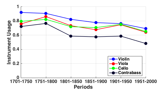
Figure 1. Instrumentation presence (left) and instrument usage (right) for string instruments.
Figure 2 reports corresponding results for woodwind instruments. In Figure 2(a) we can see that three woodwind instruments—oboe, flute, and bassoon—are most commonly included in the instrumentation. By the 19th century, the clarinet—newly developed from its predecessor, the chalumeau—joined these three core woodwinds. Notice that the oboe was the most popularly included woodwind instrument in the 18th century. Referring to Figure 2(b) we can see that oboe, flute, bassoon and clarinet tend to sound at least 40% of the time (with an exception for the flute in 1751–1800). After 1800, flute, oboe, clarinet and bassoon are roughly equivalent in use, although clarinet and bassoon sound more often than flute and oboe. When present, the bassoon has tended to be the most active of all woodwinds.
Four other woodwinds—piccolo, English horn, bass clarinet, and contrabassoon—follow a separate though similar trajectory, showing increased prominence in the late 19th century. However, even when present, these instruments tend to be used more sparingly, typically between 20–40% of the time. (The apparent exception of the English horn around 1801–1850 is probably spurious due to a small sample size—see Figure 2(a).) Of these specialty woodwinds, the piccolo has been the most popular addition in terms of the instrumentation presence, yet both piccolo and contrabassoon are used more sparingly than English horn and bass clarinet. In general, the data presented in Figure 2 are consistent with the existence of a core group of woodwind instruments consisting of oboe, flute, bassoon, and clarinet, with other woodwinds serving secondary or specialty roles.
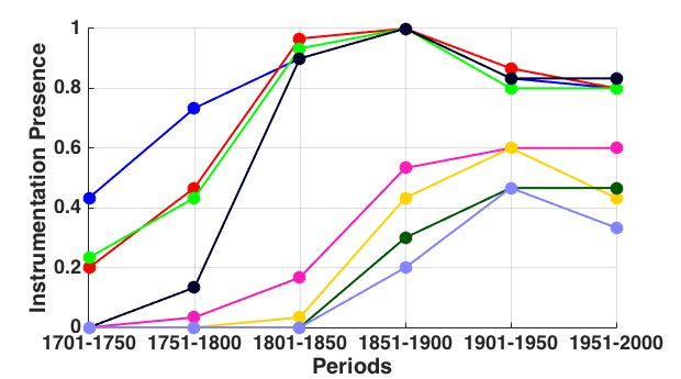
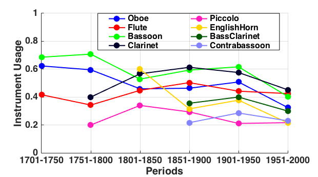
Figure 2. Instrumentation presence (left) and instrument usage (right) for woodwind instruments.
The instrumentation and usage patterns for brass instruments are shown in Figure 3. Note that the French horn is the most popular brass instrument in both instrumentation presence and instrument usage. With the exception of French horn and trumpet, the brass instruments exhibit rather stable instrument usage patterns, which might suggest that the compositional intention for using a brass instrument changed little over time. In general, high-pitched brass instruments have been favored over low brass.
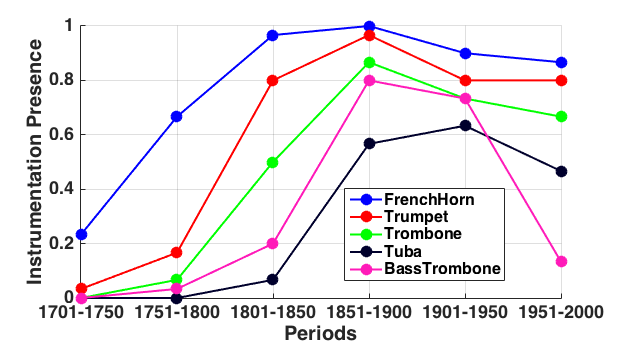
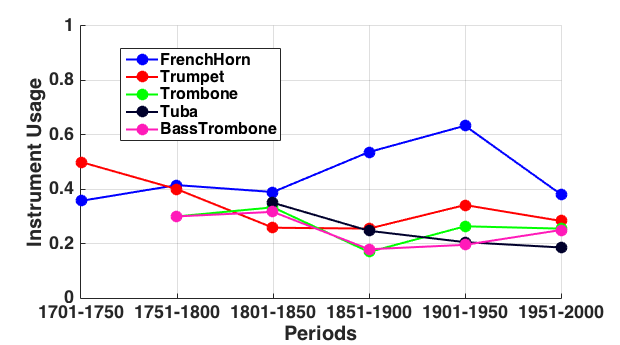
Figure 3. Instrumentation presence (left) and instrument usage (right) for brass instruments.
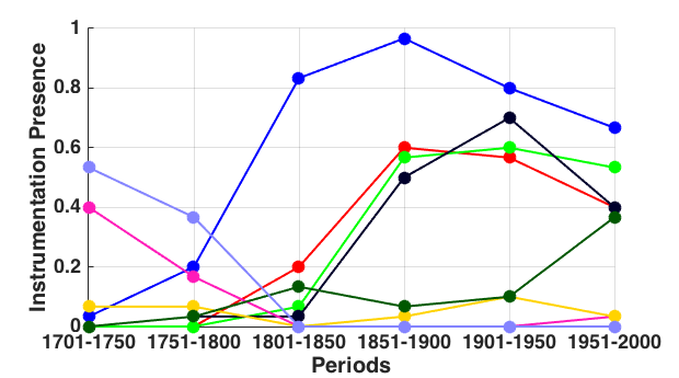
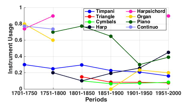
Figure 4. Instrumentation presence (left) and instrument usage (right) for percussion and keyboard instruments.
Figure 4 presents instrumentation presence and instrument usage patterns for keyboard and percussion instruments. Most noticeable is the predominance of the timpani in the instrumentation presence. Throughout the late 19th century, the timpani was present in nearly all orchestral works we sampled. The timpani is also notable for sounding in around 20% of the sampled sonorities. The presence of cymbals and triangle are notably common after the mid 19th century, although their usages are roughly half that of the timpani.
As one would expect, there is a rapid disappearance of the harpsichord and continuo at the end of the 18th century. However, the piano remains something of a rarity in orchestral music—included much less often than an instrument like the harp. When the piano is included in the instrumentation, its usage declines dramatically from the early 19th century to the mid 20th century. That usage trend reverses in the late 20th century. Notice also that by the late 20th century, the piano is as frequently included in orchestral score as was the harpsichord in the early 18th century.
Of course, instruments wax and wane in popularity. In order to determine the most prominent changes, we identified 20 instruments whose instrumentation presence showed the greatest variance (or standard deviation) across successive 50-year epochs. The pertinent boxplots of instrumentation presence are plotted in Figure 5, in order of decreasing variances from left (clarinet) to right (oboe). The box for each instrument shows the 25−75% range of the values and the whiskers designate the range of ±2.7 standard deviations (99.3 percentile coverage assuming normal distributions). The red bars within boxes specify the median values and red crosses outside boxes identify outliers. Note that the ranges specified by whiskers are in general but not exactly in a decreasing order. This is a consequence of the fact that data for individual instruments are not normally distributed. In fact, the data plotted for each instrument in Figure 5 consists of just six points, one for each epoch. The non-normal distributions explain why many of the median values (red bars) are not positioned near the center of the boxplots.
Examining the 20 instruments' presence patterns in Figure 5, we see that these are mostly percussion and wind instruments. In fact, none of the string instruments (violin, viola, cello, and contrabass) are included here, presumably because they have consistently formed the core of the orchestra from the earliest years. The instrument exhibiting the largest variance is the clarinet. This likely reflects the fact that it was introduced later than most woodwind instruments yet quickly became a common member of the orchestra. Similarly, the inclusion of continuo can be explained by its disappearance from orchestral music after the 18th century. It is also notable that Figure 5 includes many instruments that play "extended" ranges, such as piccolo and contrabassoon, as well as percussion instruments (such as triangle and timpani), all of which are generally reserved for some occasional specific effects.
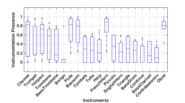
Figure 5. Boxplot of 20 instruments with the greatest variability in instrumentation.
In contrast to the instruments with the greatest variability in orchestration, Figure 6 shows the 20 most commonly included instruments over the 300-year period of this study. In other words, these instruments show the highest averages in terms of their presence in instrumentation. As in Figure 5, boxes and whiskers represent the distributions of instrumentation presence. The blue dots denote the mean values, which are all connected by a solid blue line for ease of reading. As expected, the four string instruments are the most common to appear in orchestral music, followed by core wind instruments (oboe, French horn, flute, bassoon, trumpet and trombone). The trombone seems to reside at a pivotal point where there is a noticeable decline in instrument inclusion. Sandwiched between the timpani (included in roughly 60% of scores) and the piccolo (included in roughly 35% of scores), the trombone is evident in just under 50% of our sample of orchestral works. The instruments below the trombone include an eclectic mix of percussion plus the more commonly used specialty instruments. Comparing Figures 5 and 6, one might wonder why certain instruments appear in both. This is not a mistake: Figure 5 shows the instruments with largest variances whereas Figure 6 shows those with largest means. Hence, some instruments such as oboe are present in both figures.
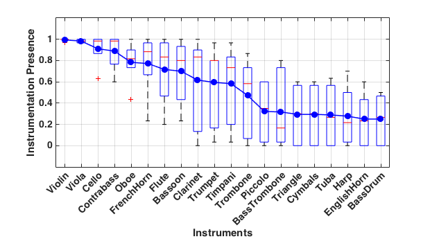
Figure 6. Boxplot of 20 instruments most commonly included in instrumentation.
Ensemble Size
Apart from changes in the use of different instruments, we might expect ensemble size to have changed over time. Our sample includes no coding of the total number of instruments in a given ensemble. We have access only to the number of notated parts—some of which may be played by multiple instruments in unison. Nevertheless, we can tally the size of the instrumentation—that is, the number of notated parts as an estimation of the ensemble per se—and study a general trend. Figure 7 shows the instrumentation size for each of the 180 sampled orchestral pieces. Each dot represents a musical score, with the corresponding composition (or publication) year and the total number of parts specified in the piece. A continuous growth in the total number of notated parts can be observed from 1700 until about 1900. Notice that there are very few samples from the period roughly 1930−1945, corresponding to the Great Depression and World War II. The associated economic hardships might have encouraged a resurgence of smaller-scale orchestral music.
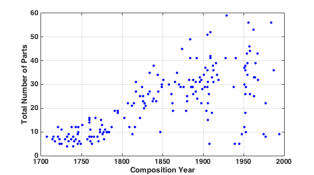
Figure 7. Total number of parts specified in orchestral scores plotted against year of composition, showing a general growth in instrumentation over time.
Figure 8 plots means (blue bars) and standard deviations (yellow bars) in instrumentation size for the six 50-year epochs. This figure shows more clearly the pattern evident in Figure 7. First, instrumentation size grows continuously over time, although the rate of increase in instrumentation size decreases dramatically from the mid 19th century. In the 20th century, there is simultaneously a tendency for composers to employ a greater variety of instrumentation sizes (as evident in the increased variances).
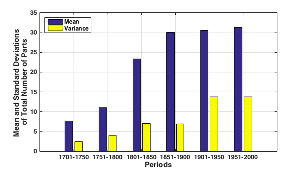
Figure 8. Means and standard deviations of the total number of parts specified in orchestral scores for each 50-year epoch, showing dramatic growth in instrumentation size until around 1850, followed by increasing variability in the 20th century.
Most Common Instrument Combinations
Some instrumental combinations are more common than others. Table 3 identifies the 16 most common instrument combinations across the entire 300-year corpus. Combinations represent sounding instruments in sonorities rather than instrumentation for the entire piece. Multiple instances of the same instrument in one line indicate that the sonorities involve multiple notated parts employing the same instrument. As can be seen, the most common combination consists of the complete string section, involving two violin parts, viola, cello, and contrabass. With the exceptions of piano solos (17 sampled sonorities) and violin solos (14 sonorities), nearly all of the patterns in Table 3 involve various combinations of the five string parts.
| Number of instances | Instrument combination pattern |
|---|---|
| 67 | violin + violin + viola + cello + contrabass |
| 27 | violin + violin + viola + cello + contrabass + oboe + oboe |
| 20 | violin + violin + viola + cello + contrabass + harpsichord |
| 19 | violin + violin + viola |
| 19 | violin + violin |
| 19 | violin + violin + viola + cello |
| 18 | violin + violin + viola + continuo |
| 17 | piano |
| 14 | violin |
| 12 | violin + violin + viola + cello + contrabass + bassoon |
| 10 | violin + violin + violin + viola + cello + contrabass |
| 10 | violin + violin + continuo |
| 10 | cello + contrabass |
| 9 | violin + violin + violin |
| 9 | violin + violin + viola + cello + contrabass + piano |
| 9 | violin + violin + viola + cello + harpsichord + continuo |
| Epoch | Number of instances | Instrumentation pattern |
|---|---|---|
| 1701 – 1750 | 19 | violin + violin + viola + cello + contrabass + harpsichord |
| 15 | violin + violin + viola + continuo | |
| 14 | violin + violin + viola + cello + contrabass + oboe + oboe +bassoon | |
| 1751 – 1800 | 27 | violin + violin + viola + cello + contrabass |
| 13 | violin + violin + viola + cello + contrabass + oboe + oboe + bassoon | |
| 9 | violin + violin + viola + cello + contrabass + harpsichord + continuo | |
| 1801 – 1850 | 10 | violin + violin + viola + cello + contrabass |
| 9 | piano | |
| 7 | violin + violin + viola + cello + contrabass + piano | |
| 1851 – 1900 | 4 | violin + violin + viola + cello |
| 3 | violin | |
| 3 | violin + violin + viola + cello + contrabass | |
| 1901 – 1950 | 17 | violin + violin + viola + cello + contrabass |
| 6 | violin + viola + cello + contrabass | |
| 5 | violin + violin + viola + cello | |
| 1951 – 2000 | 5 | piano |
| 4 | violin + violin + violin + violin + viola + viola + cello + contrabass | |
| 3 | violin + violin + viola + cello + contrabass | |
| 3 | cello | |
| 3 | harp |
Table 4 provides comparable information for each 50-year epoch—focusing on the three most common instrumental combinations. The most popular five-part string combinations are found in every epoch except for the early 18th century (which shows three variations of the five-part string combination). Also noticeable is the general decline in the number of sampled sonorities for each instrumental combination over the three centuries spanned by our corpus. This likely reflects the fact that composers tend to incorporate more instruments in their compositions over time, which in turn enables a greater range of instrument combinations.
Apart from instrument combinations, of further interest are the usage patterns of specific instrument pairs. In studying how instruments tend to be paired with other instruments, cluster analysis provides a useful approach as it identifies grouping pattern at various hierarchical levels. Although it might prove interesting to consider the hierarchical clustering patterns of all 91 instruments, since many of these instruments rarely appear in our sample, we would expect a large uninformative grouping consisting of rarely used instruments. A more informative approach might begin by simply excluding the less common instruments, and concentrating on the most common ones. Accordingly, we began by selecting those instruments that appear in the majority of orchestral scores: flute, oboe, clarinet, bassoon, French horn, trumpet, trombone, timpani, violin, viola, cello, and contrabass. Recall that Johnson (2011) also carried out cluster analysis of instrument pairings. In order to facilitate direct comparison with his results, we chose to add eight additional instruments that were included in Johnson's analysis: piccolo, English horn, bass clarinet, contrabassoon, bass trombone, tuba, harp, and cornet. Consequently, our analysis focused on these 19 of the 91 instruments present in our sample. Inter-instrument distances were defined as the reciprocal of the number of instrument pairings in our sample of sonorities. More specifically, we divided by 1,800 the total number of instances for each pair of the 19 instruments, and then subtracted this ratio from 1. The resulting numbers consequently provide a distance metric, with more frequently used instrument pairs exhibiting values closer to 0. Cluster analysis was carried out on these distances employing Ward linkage with Euclidean distance in SPSS.
Four analyses were carried out representing the hierarchical clustering of instruments for each of three centuries (18th, 19th, and 20th), as well as for the entire 300-year span. Figure 9 shows the result for the 18th century. Five instruments (contrabassoon, cornet, bass clarinet, English horn, and tuba) were excluded from the analysis due to their rarity at the time. Harp and clarinet were retained in the analysis because they started making an appearance in orchestral music in the late 18th century. At the highest level, two groups are evident, with the strings distinguished from all of the other orchestral instruments. This division probably reflects the fact that much music in the 18th century was composed for string orchestra. At a clustering distance of around "5," three main clusters are evident: Strings (violin, viola, cello, and contrabass), Core Winds (bassoon, French horn, flute, and oboe), and what might be dubbed Effects (piccolo, harp, trombone, trumpet, timpani, and clarinet). The Effects instruments were so very rarely used that they did not form any sub-clusters within the cluster. The Strings cluster shows two sub-clusters: violin-viola and cello-contrabass. These pairings likely reflects the practice that the viola tended to double the violin, whereas the contrabass tended to double the cello in the 18th century.
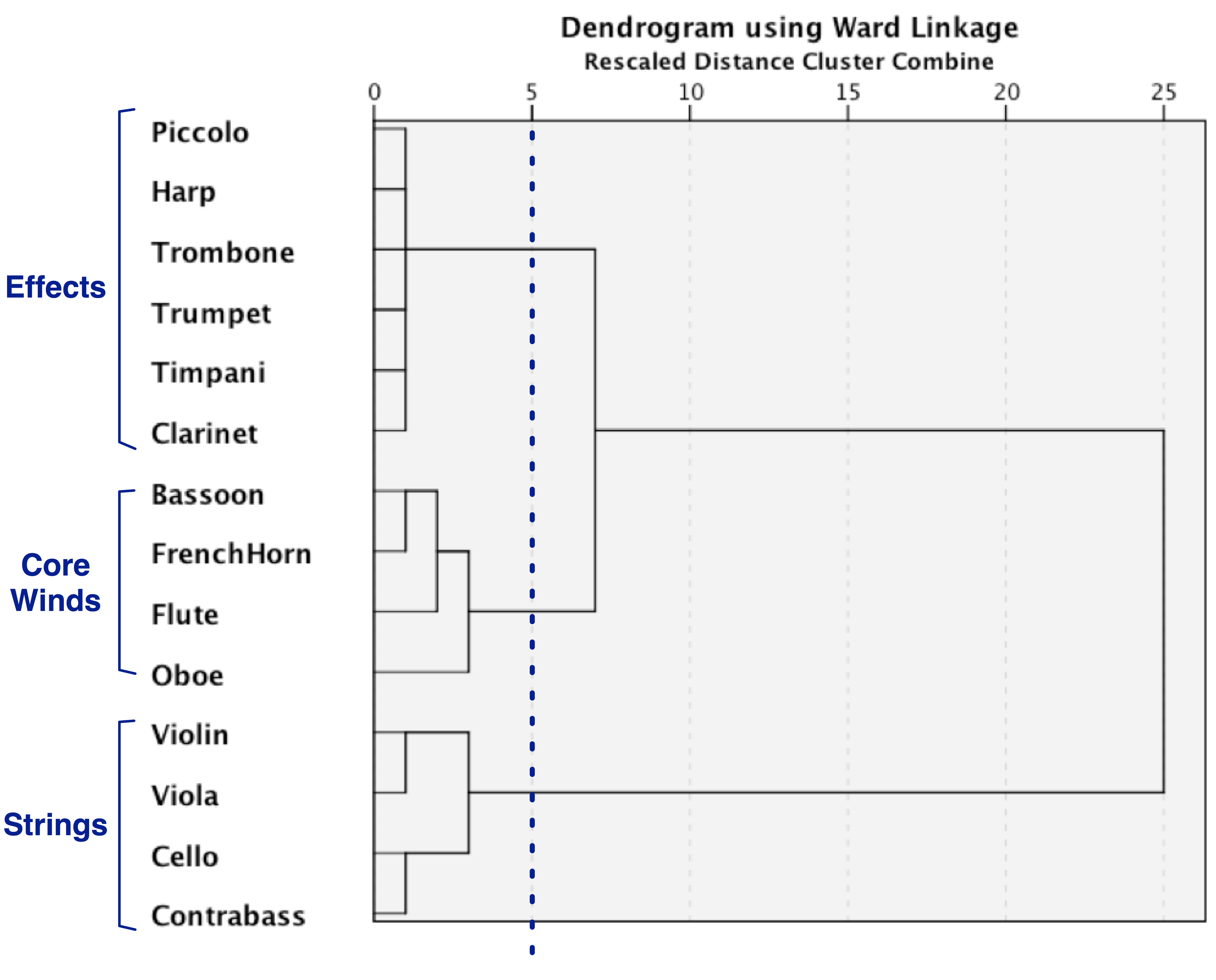
Figure 9. Hierarchical clustering of typical orchestral instruments in the 18th century showing three main clusters dubbed Strings, Core Winds, and Effects.
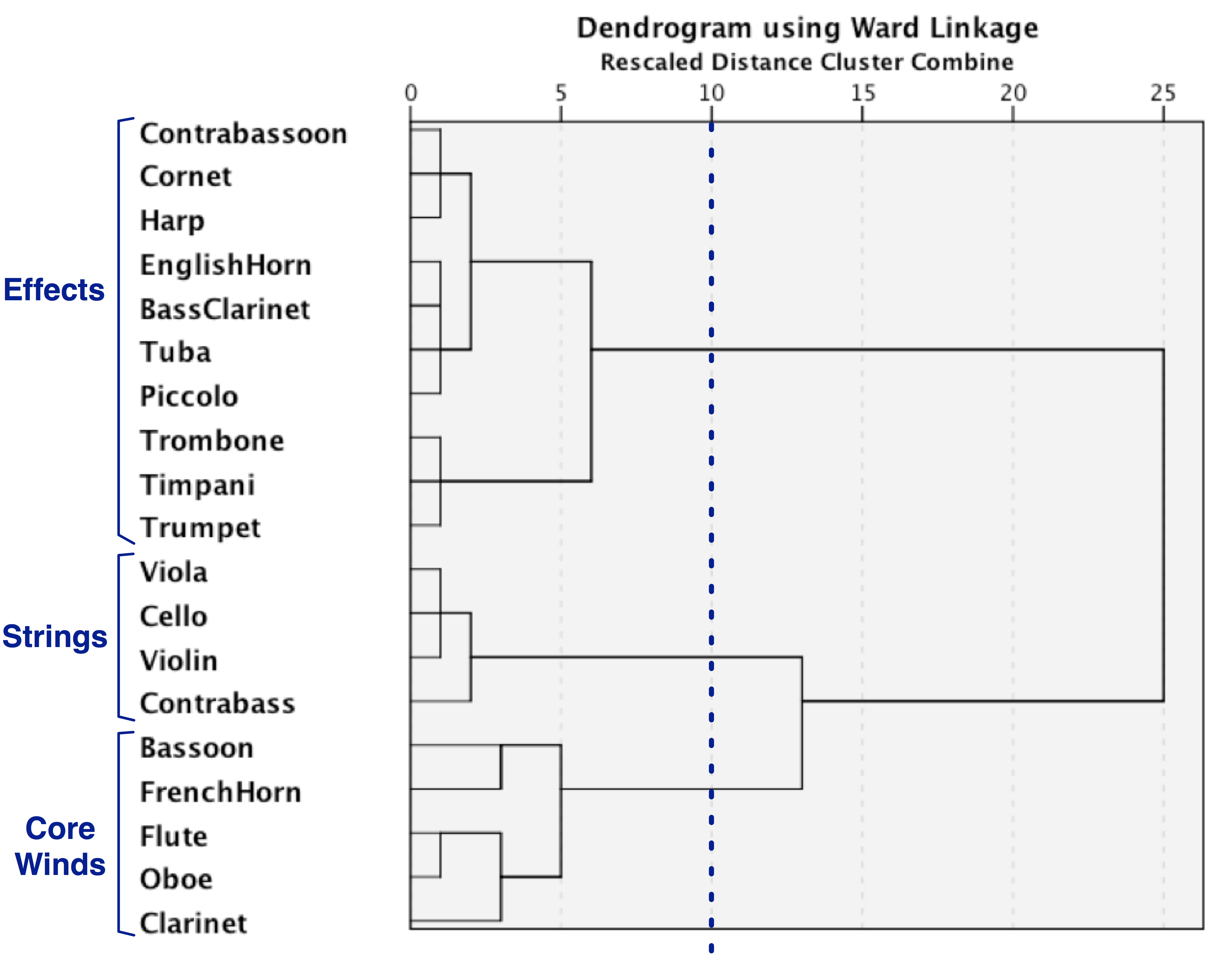
Figure 10. Hierarchical clustering of typical orchestral instruments in the 19th century showing three main clusters dubbed Strings, Core Winds, and Effects.
Figure 10 presents the result of hierarchical clustering analysis for the 19th century, using all 19 instruments. At the top level we see two large clusters. The lower group of nine instruments corresponds to Johnson's Standard group (with the notable addition of the French horn). The upper group of 10 instruments might simply be deemed "non-standard" instruments. At the clustering distance of "10," we again see three overarching clusters: Strings (violin, viola, cello, and contrabass), Core Winds (bassoon, French horn, flute, oboe, and clarinet), and Effects (contrabassoon, cornet, harp, English horn, bass clarinet, tuba, piccolo, trombone, timpani, and trumpet). In the Core Winds cluster, we see the same four instruments evident in the 18th century; however, we also see that the clarinet has made the transition from the Effects cluster in the 18th century to the Core Winds in the 19th century. Within the Effects cluster, we see three sub-clusters. These sub-clusters appear to reflect the overall frequency of use. Of the ten instruments in the Effects cluster, trumpet, timpani, and trombone are undoubtedly the most commonly used. A second sub-cluster (tuba, piccolo, bass clarinet and English horn) appears to represent less commonly used instruments. The third sub-cluster includes the least commonly used of the Effects instruments (harp, contrabassoon, and cornet). In the case of the most frequent of the Effects sub-clusters, we see what might be dubbed a "proto-power" group (trumpet, timpani, and trombone), which in Johnson's study would have expanded to include the tuba and piccolo, as well as the French horn. Compared with the 18th century, the 19th-century Effects cluster has expanded considerably—presumably reflecting composers' interests in extending both the pitch range of the orchestra and the dynamic range (especially for louder textures).
Notice that in both 18th and 19th centuries, the Strings cluster includes two sub-clusters. However, the partitioning of the instruments is different. In the 18th century, the cello and contrabass form one group with the violin and viola forming a second group. By contrast, in the 19th century, the cello is grouped with violin and viola, with the contrabass forming its own separate cluster. It is possible that the yoking together of cello and contrabass in the 18th century is a legacy of figured bass practice. In the 19th century, rather than simply constantly doubling the cello, the contrabass appears to have achieved some functional independence.
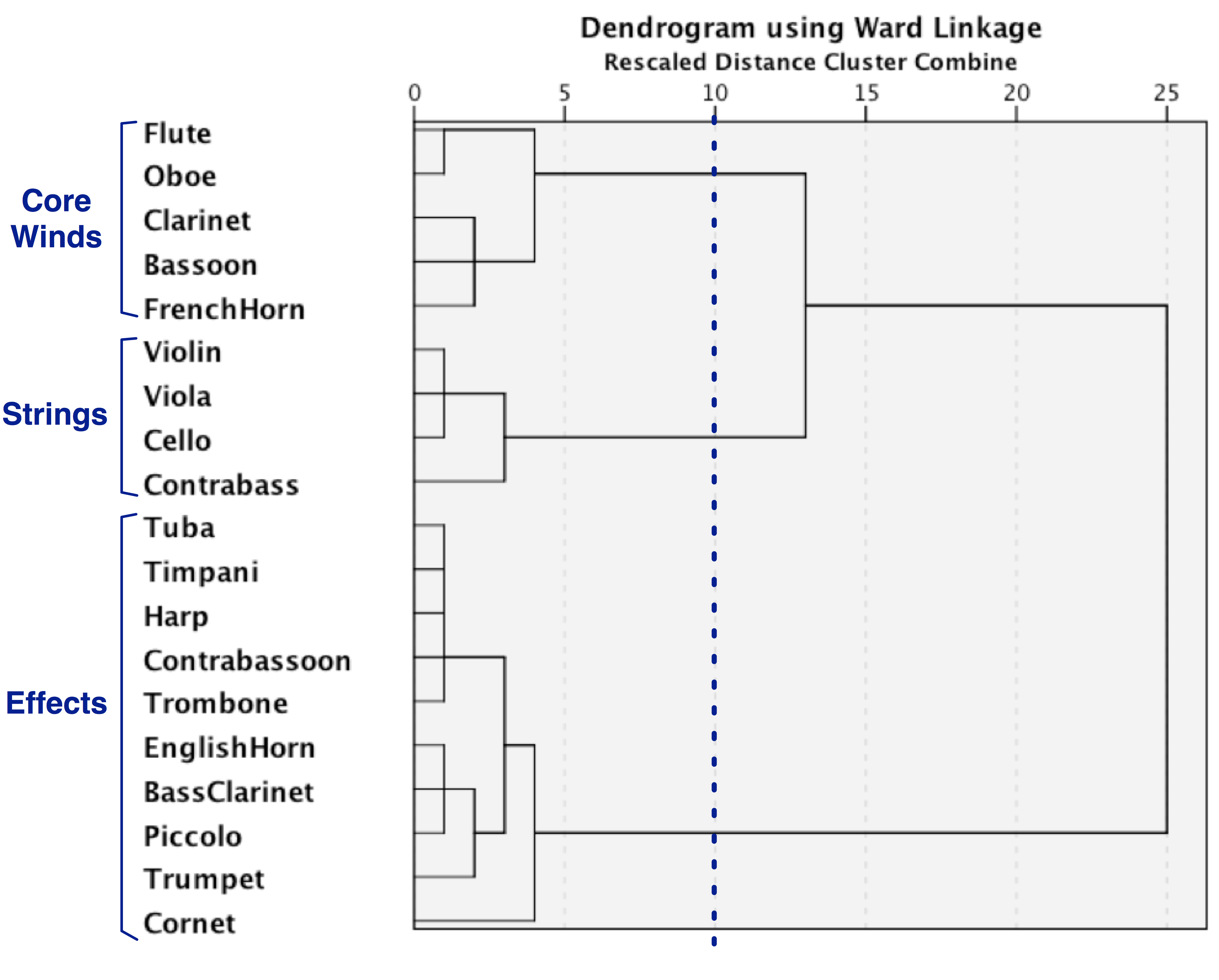
Figure 11. Hierarchical clustering patterns of typical orchestral instruments in the 20th century showing three main clusters dubbed Strings, Core Winds, and Effects.
Figure 11 displays the results for the 20th century. At the top-most level, we again see two clusters that might be deemed Standard and Non-standard instruments in accordance with Johnson (2011). At a clustering distance of "10," we see the same three clusters observed in the earlier figures: Core Winds (flute, oboe, clarinet, bassoon, French horn), Strings (violin, viola, cello and contrabass), and Effects (all the other instruments). The Strings cluster shows the same within-cluster pattern as in the 19th century—with the contrabass somewhat independent of the violin-viola-cello group. The Core Winds cluster exhibits two sub-clusters that appear to simply distinguish high-pitched instruments (flute and oboe) from lower-pitched instruments (clarinet, French horn and bassoon). Within the Effects cluster, the cornet is first isolated from the others—presumably reflecting its relative rarity. The remaining two sub-clusters within the Effects group are vaguely reminiscent of Johnson's Power and Color groups, however the groups in our 20th-century sample are much more diffuse. The 20th-century version of the "proto-power" sub-cluster appears to consist of the tuba, trombone, contrabassoon and timpani, plus the harp. With the exception of the harp, this proto-power sub-cluster emphasizes low-and-loud instrumentation. In contrast with Johnson's Power group, the trumpet and piccolo have been assigned to a different sub-cluster that contains other instruments more reminiscent of Johnson's Color group. This might imply that the "power" sound in the 20th century emphasizes a darker overall texture. Alternatively, one might regard this as evidence that 20th-century composers distinguish "dark power" from "bright power"—although the inclusion of the English horn and bass clarinet suggests that "bright power" may be a questionable interpretation.
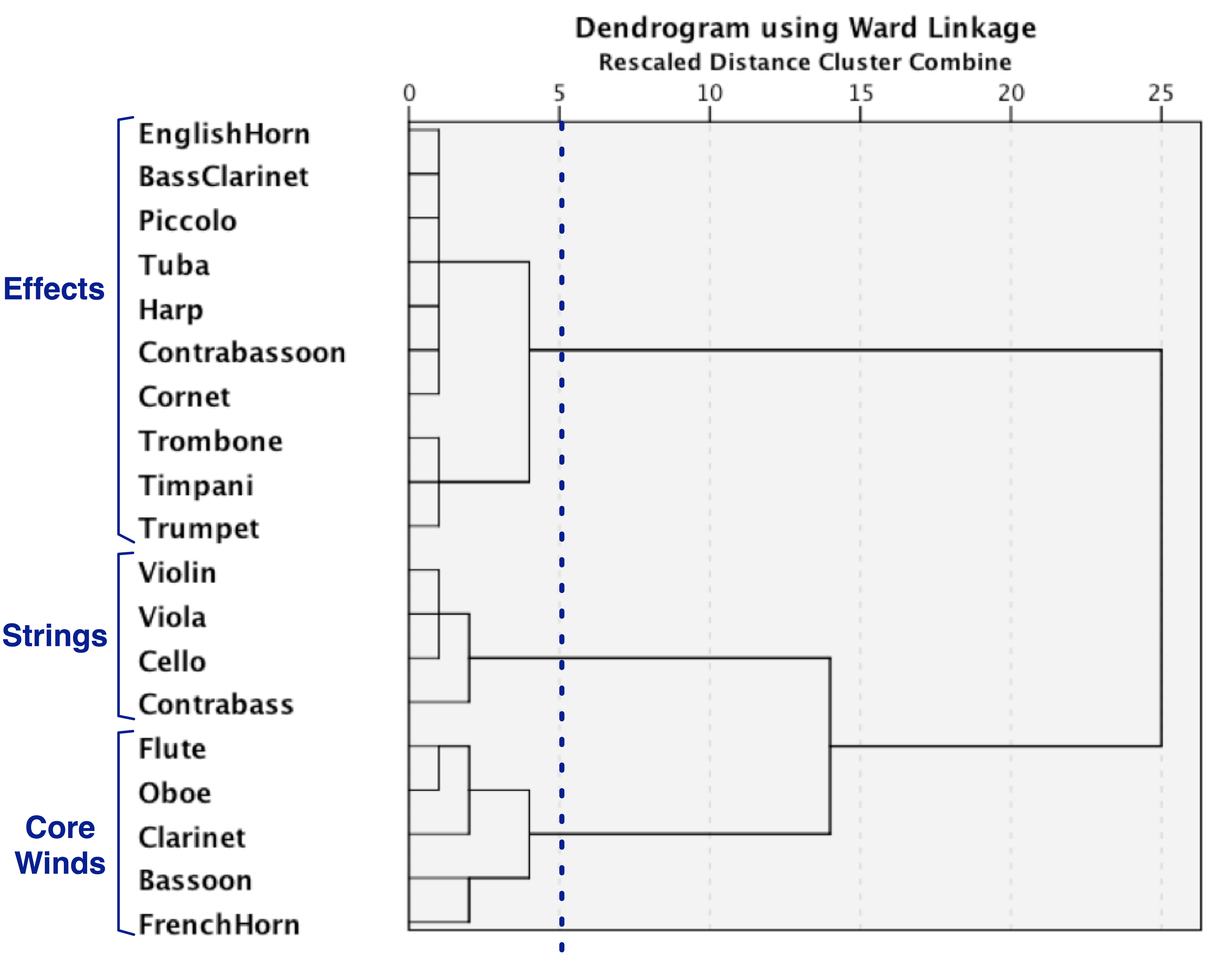
Figure 12. Hierarchical clustering of typical orchestral instruments over 300 years (1701–2000), showing three main clusters dubbed Strings, Core Winds, and Effects.
Figure 12 shows the clustering patterns found across the entire corpus spanning three centuries. Overall, we see the same three clusters, dubbed Strings, Core Winds, and Effects. As noted earlier, the separation of the contrabass from the rest of the string instruments probably reflects its increasingly independent function, rather than simply doubling the cello. The two sub-clusters in the Core Winds group seems to imply functional differences: flute and oboe exhibit higher pitch ranges; the clarinet exhibits a middle pitch range; all three of these woodwinds are more likely to play a foreground role, whereas bassoon and French horn exhibit lower pitch ranges and are more likely to perform background functions. The Effects cluster divides into two sub-clusters: a nascent "proto-power" sub-cluster consisting of trumpet, trombone, and timpani, and a second sub-cluster of the remaining "occasional-use" instruments.
Having identified various instrumental groupings, we might consider how well these groupings have maintained their cohesion over the 300-year span of our study. By "cohesion", we mean the within-group instrument combinations. Are there any general trends that emerge across history? In light of the extant research, we have at least three different ways of classifying groups of orchestral instruments. One classification follows the clustering study by Johnson—the Standard-Power-Color groupings. A second classification follows from our own clustering study—the Strings-Core Winds-Effects groupings. Finally, a third classification might simply follow the traditional instrument "families" designations—Strings-Woodwinds-Brass-Percussion. In the ensuing analyses, we trace how well the instruments in these various groupings retain their affinity for each other across history. As a measure of group cohesion, we tally the total number of intra-group instrument pairings for each epoch divided by the total number of instrument pairings (both intra- and inter-group). The results are presented in Figures 13 through 15, where each figure reports the historical changes for a different system of instrument classification. We begin with instrument families grouping.
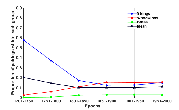
Figure 13. Proportion of within-group instrument pairings by instrument family through six epochs.
Figure 13 shows the proportion of instrument pairings within each instrument family (strings, woodwinds, brass). The percussion family is missing because only one of the 19 common instruments is a percussion instrument (timpani). The most notable feature evident in Figure 13 is the marked reduction of cohesion among the strings. The strong affinity among string instruments in the 18th century is perhaps an artifact arising from the fact that many early orchestras consisted predominately of strings. In contrast to the string family, the woodwinds rise continuously in their mutual association from 1700 to the mid 19th century. From the mid 19th century onward, the cohesiveness of the woodwind family rivals (and even exceeds) the cohesion of the strings.
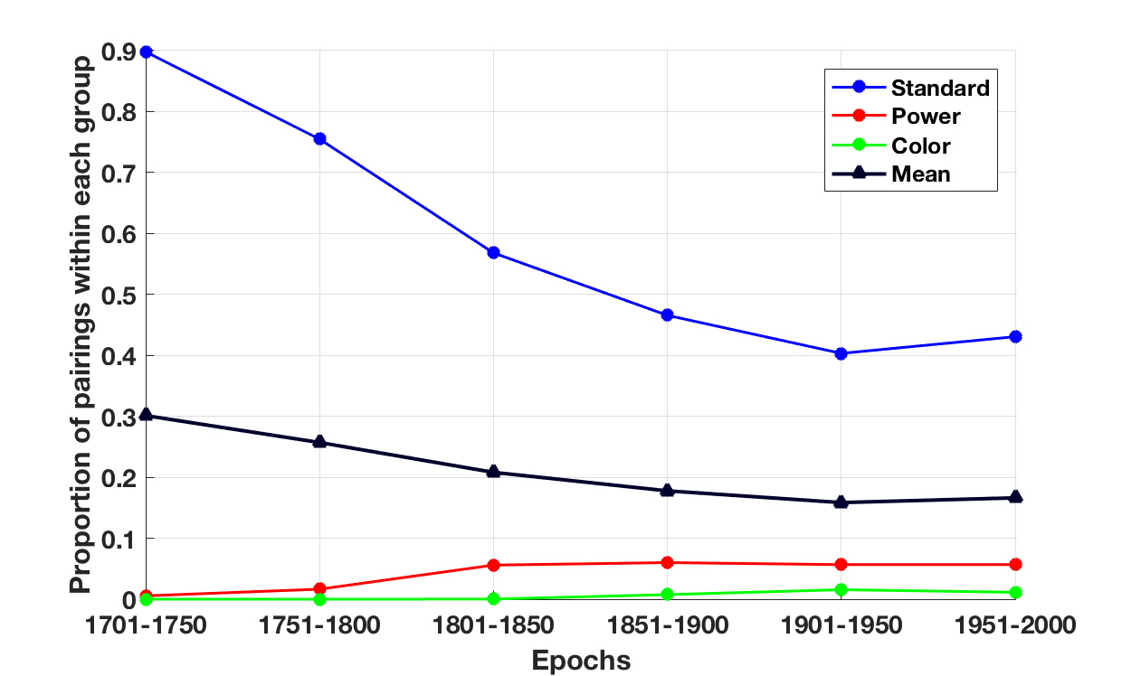
Figure 14. Proportion of within-group instrument pairings according to Johnson's Standard-Power-Color functions through six epochs.
Figure 14 plots comparable changes in the mutual association for Johnson's Standard-Power-Color instrument groupings. Notice first the dramatic decline in the cohesion of the Standard instrumental group. This group includes flute, oboe, clarinet, bassoon, violin, viola, cello, and contrabass. The decline of the Standard instruments resembles the decline of the String family in Figure 13; however, where the decline in String cohesion levels off around 1800, the decline of the Standard instruments continues until the early-mid 20th century. Only at the end of the 20th century do we see some recovery in the mutual association of the Standard instrumental group. The Power instruments (piccolo, trumpet, trombone, French horn, tuba, and timpani) remain rather dispersed, but nevertheless gain in cohesion from the 18th century to the 19th century.
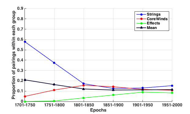
Figure 15. Proportion of within-group instrument pairings by the Strings-Core Winds-Effects model through six epochs.
Figure 15 presents the cohesion (within-group proportion-pairings) using the Strings-Core Winds-Effects model arising from our own hierarchical clustering analysis. The results strongly resemble the family-based groupings plotted in Figure 13. The Strings group (blue line) is necessarily identical to the String group in the family-based analysis. The Core Winds also exhibits a similar behavior to the Woodwind group in the family-based analysis. Compared with the Woodwind family, recall that our Core Winds group includes the French horn and excludes piccolo, English horn, bass clarinet, and contrabassoon). Notice, however, that our Core Winds peaks earlier (1801–1850) than the Woodwind family (1851–1900). Finally, in contrast to the behavior of the Strings and Core Winds, the Effects group shows a constant growth in cohesion throughout the six epochs, although it may have reached a plateau around the mid 20th century.
Notice that all three models—the instrument family model, the Standard-Power-Color model, and the Strings-Core Winds-Effects model—show a similar longitudinal pattern. All three show a rapid reduction in the cohesiveness of the Strings or Standard instrumentation through the 18th century. In the 19th century this decline abates somewhat (although the Standard instrumentation continues to exhibit a decline in the mutual association of these instruments). At the same time, there is a modest increase in the cohesion of other groups (woodwinds/brass/power/effects instruments). This growth concurs with traditional historical observations that successive generations of composers continued to pursue novel sounds, both by incorporating new instruments into the ensemble, and by using unprecedented instrument combinations. Interestingly, in all three models, there is an apparent up-tick in cohesiveness in the latter half of the 20th century, although it may not be statistically significant.
In characterizing changes in the mutual association of instruments, the above results all relied on specific models of instrument groupings. However, there is a more direct way of measuring the variety of instrument pairings or affinities. A useful tool for characterizing variety is to measure entropy using the classic information theory equation from Shannon and Weaver (1949). An advantage of this approach is that it does not rely on the a priori clustering models used above. Entropy (H) is defined as follows:

where X is a discrete random variable with n possible values {x1, x2, …, xn} and P(X) is the probability mass function of X. In our case, X will be the possible instrument pairing with 4,095 (= 91 choose 2 = 91×90/2) possibilities and P(X) will be the actual proportion of occurrences of each specific pairing. When there is little variety (and therefore less uncertainty), the entropy value will be smaller; when there is more variety, the entropy value will be larger.
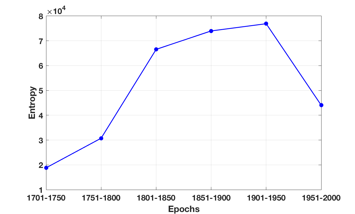
Figure 16. Change in entropy for paired-instrument combinations through six epochs.
Figure 16 shows the change in entropy for paired-instrument combinations through six epochs. Remember that Figures 13 through 15 were obtained by considering the instrument pairing patterns of the 19 typical orchestral instruments. However, the entropy values plotted in Figure 16 were obtained using the entire list of 91 instruments found in our data set. Of course, many of these 91 instruments were not used in the 18th century. Since the number of possible instrument pairing patterns was more limited (and more homogeneous), we would expect low entropy values for the early 18th century. In later periods, we observe higher entropy values consistent with more diverse possibilities for instrument pairings.
What is unexpected in Figure 16 is the large drop in entropy in the late 20th century. This result suggests that the number of unique combinations of instrument pairs declined dramatically in the late 20th century. Notice that this particular decline in entropy is lower than comparable values for the entire 19th century. There are several possible reasons why such a low entropy value might arise. It is possible that this unusual value is simply an artifact of unlucky or unrepresentative sampling. Given the sample size (300 sonorities from 30 works), this is possible but unlikely. At face value, the result suggests that late 20th century composers employed more restricted or fixed palette of instrument combinations. At least four causal conjectures might be considered.
One possibility is that the low entropy arises due to a smaller ensemble size. In principle, a work written for ten instruments offers many more possible combinations than a work written for five instruments. However, with respect to the number of musical parts, Figure 7 suggests that there is little or no difference in the pertinent distributions between early and late 20th centuries. An independent-samples t-test confirms that the first half of the 20th century (M = 30.6, SD = 13.7) did not differ significantly from the later half (M = 31.3, SD = 13.8) in terms of the total number of parts specified in the scores (t(58) = −.197, p = .844, d = .05). Alternatively, early and late 20th centuries might differ with regard to the number of unique instruments used. For example, two works might both entail ten notated parts; however, if one work is written for ten different instruments and the other work is written for five pairs of different instruments, then the latter work is likely to exhibit lower entropy for instrument combinations.
A second possibility is that late 20th century composers reverted to more traditional instrument combinations. Although this is possible, it seems unlikely since the palette of instruments used in this epoch remains strikingly broad compared with earlier centuries. A third possibility is that late 20th century composers made greater use of repetition—returning to the same instrument combinations again and again. This suggestion is consistent with the rising popularity and prominence of Minimalism in the latter half of the 20th century, although our late 20th century sample included only one minimalist work.
Finally, we need to reconcile the dramatic decline in entropy with the results plotted in Figures 13–15. One might have expected that, given the remarkable drop in entropy, the instrument groupings in our three clustering models would also show a correspondingly dramatic rise. There is a noticeable up-tick in the proportion of instrument pairings in the Standard instruments in Figure 14, as well as a slight discernible increase in the cohesion of the strings in both Figures 13 and 15. At the same time, there are overall creeping increases in the mutual association of Woodwinds, Brass, and Effects groupings. However, these increases are small in comparison to the entropy decline for the late 20th century. At face value, the results suggest that late 20th century composers made use of stable recurring combinations of instruments, but that these combinations did not coincide with traditional instrument groupings, such as by instrument family. That is, orchestration in the late 20th century appears to be characterized by a form of predictable uniqueness or standardized novelty. Tracking down the origin of this apparently dramatic change in entropy is likely to require a major project in itself and is beyond the scope of the current study.
Dynamics
With regard to dynamics, we might consider which instruments are most likely to play at different dynamic levels. Each instrument's usage was tallied for each of ten dynamic levels (ffff, fff, ff, f, mf, mp, p, pp, ppp, pppp) as well as dynamic changes of crescendo and decrescendo. In our analysis, we focused on 16 core orchestral instruments (violin, viola, cello, bass, flute, piccolo, oboe, English horn, clarinet, bassoon, French horn, trumpet, trombone, tuba, timpani and harp). The results are presented in Figure 17. The color of each cell corresponds to the number of samples found for that category—the mapping of which is given to the right of the figure. Darker luminance indicates higher values. As can be seen, the extreme dynamic levels (such as ffff and pppp) are rarely used. In general, there is a bias towards loud dynamic markings over quiet dynamic markings. For example, the dynamic markings ff, f, and mf are more common than their quiet counterparts, pp, p, and mp. Notice that this asymmetry does not necessarily mean that loud dynamic levels predominate in orchestral music. Dynamic markings are relatively sparse in musical scores and so may represent marked states—the exceptional rather than the commonplace or normal (unmarked) state. One cannot dismiss the possibility that the predominance of loud markings might arise because most musical passages are assumed to exhibit a relatively subdued dynamic level.
In general, string instruments are used more often than woodwinds, which in turn are used more frequently than brass or percussion instruments. It is interesting to observe that the usage of the French horn appears to follow the woodwinds (flute, oboe, clarinet, bassoon) rather than other brass instruments. This pattern is in agreement with what Adler (2002, p.296) observes: "The brass choir, which is more homogeneous than the woodwind section, is often divided into two groups: 1. The horns; 2. The trumpets, trombones, and tuba. This division reflects the different use the horns have from other brass instruments; in addition to being part of the brass choir they have been employed as adjuncts to the woodwind section because of their unique ability to blend with and strengthen the woodwind sound." This unique pattern of the French horn separate from other brass is in agreement with the results from our hierarchical clustering which grouped the French horn with the flute, oboe, clarinet, and bassoon into the Core Winds group. The bottom two rows of Figure 17 present the instrument usage patterns in samples taken from passages with changes in dynamics (< for crescendo and > for decrescendo).
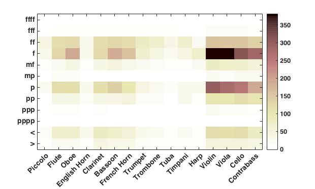
Figure 17. Count of instrument appearances according to dynamic level.
It should be noted that the tallies represented in Figure 17 are confounded by the simple frequency of occurrence for each instrument. Hence, a frequently used instrument will appear to be used frequently for a given dynamic level simply because the instrument is commonly used. Figure 18 presents the same information normalized according to instrument usage, so it is easier to compare the associations between instrument and dynamic level. In addition, Figure 18 excludes data for extreme dynamic levels (fff, ffff, ppp, pppp) and for mp since the number of data points is small. After normalization per instrument, the string instruments no longer dominate the figure. What is noticeable (and rather unexpected) is the high usage of the harp in f. Otherwise Figures 17 and 18 show similar patterns. Notice that most wind instruments (brass and woodwinds) are more likely to sound in f and ff than in any other dynamic levels. This pattern likely reflects the relative difficulty of playing quietly using wind instruments. In contrast, the strings are almost equally likely to sound either in f or p.
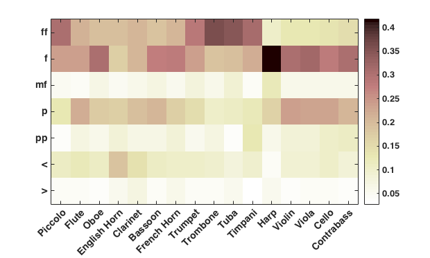
Figure 18. Proportion of instrument usage for each dynamic level from pp to ff as well as crescendo or decrescendo (after normalization per instrument).
In the same way that instruments appear with different frequencies, dynamic levels also appear with different frequencies. Consequently Figure 18 is dominated by values for p, f, and ff. With regard to changing dynamics, notice that the decrescendo row exhibits a consistently lighter hue than the crescendo row. This simply means that our samples included more instances of crescendos than decrescendos, consistent with earlier findings regarding the dominance of crescendos (Huron, 1990a, 1990b, 1991). In order to clarify the association between instrument and dynamic level we might first normalize the data according to dynamic level. Accordingly, Figure 19 shows the proportion of instrument usage after double normalization: first, the number of samples was normalized across all instruments per dynamic level (hence, treating ff as equally likely to occur as pp). The results represent the probability of an instrument sounding in a given dynamic level. Second, this probability was again normalized by the total probability of an instrument sounding across all dynamic levels. This double normalization reveals details that are not evident in Figure 18.
Figure 19 shows once again the expected association between brass, piccolo and timpani with loud dynamic levels, especially ff passages. Quiet dynamic levels tend to be associated with the strings, especially the low strings (cello and contrabass). Notice that the timpani exhibits a marked bifurcation—it is associated with both ff passages and pp passages; the timpani rarely plays during more moderate dynamic levels. Similar though much attenuated bifurcations are evident with the French horn (pp and f/ff), the flute (p and ff), and the contrabass (pp and f). Although we did not code for articulation, we expect that the contrabass's connection with pp is likely associated with the use of pizzicato. The two instruments most associated with moderate dynamic levels are bassoon and harp. In general, the strings exhibit a rather uniform likelihood to sound across all dynamic levels, which accords with the maxim that "the strings always play." As might be expected, the strings exhibit less affiliation with ff dynamics than is the case for brass and woodwinds.
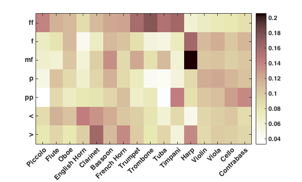
Figure 19. Proportion of instrument usage in each dynamic level from pp to ff as well as for crescendo or decrescendo (after double normalization; first per dynamic level, then per instrument).
Turning to changing dynamics, the French horn and harp have notable affiliations with decrescendo, whereas the English horn appears to have a strong affiliation with crescendos. Most importantly, the clarinet features prominently in both crescendo and decrescendo passages. In fact, the clarinet exhibits a stronger association with changing dynamics than with static dynamics. This affiliation probably reflects the instrument's remarkable dynamic range. Perhaps only the timpani can match the clarinet's ability to play both quietly and loudly. Given the sustained sound of the clarinet, it seems admirably suited to increasing or decreasing dynamics.
In comparing crescendo with decrescendo, there appears to be an association with pitch height. High-pitched instruments, like piccolo, flute, and oboe, have a greater affinity for crescendos compared with decrescendos. Conversely, lower-pitched instruments—such as clarinet, French horn, and tuba—are more likely to be associated with decrescendos than crescendos. This association implies gestures that link louder-higher and quieter-lower.
In interpreting Figure 19, one might suppose that differences in the use of specific dynamic levels (such as the marginal difference between mf and f) might tend to obscure more general trends. In addition, recall that Figure 19 omitted less frequently occurring dynamic levels such as fff and mp. In order to better glimpse possible general trends, one might employ a moving-average filter. Accordingly, Figure 20 uses a three-point moving average filter after double normalization. For example, the values plotted for f represent 60% of the original f category, plus 20% each of the flanking categories of mf and ff. In the case of the dynamic extremes (ff and pp), the moving average calculation included all of the even more extreme values as a collapsed category. In effect, ffff was re-coded as fff when calculating the moving average for ff. Similarly, pppp was re-coded as ppp when calculating the moving average for pp. This procedure was used due to the very low numbers of observations in these categories.
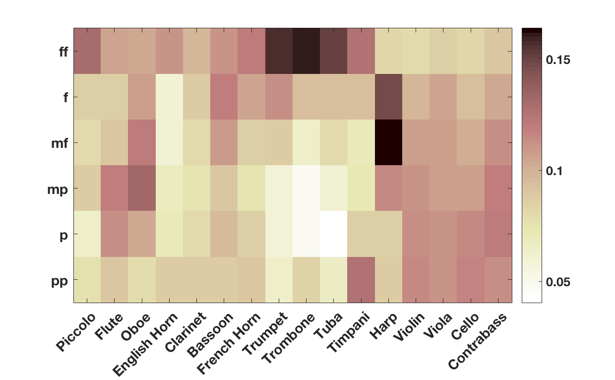
Figure 20. Smoothed (three-point moving average) proportion of each instrument's usage at each dynamic level (after double normalization; first per dynamic level, then per instrument).
In Figure 20, notice that the affinity of the contrabass for low dynamic levels is even more prominent, and is now joined by violin, viola, and cello. In general, the association of the strings with low dynamic levels is more apparent in this presentation. In addition, the lower strings show an even greater affinity for the lower dynamic levels. Once again, the affiliation of the brass (and piccolo) with loud dynamics is evident, and the timpani continues to exhibit a bimodal association with the extreme dynamic levels of ff and pp. Of the brass instruments, the trombone seems more strongly restricted to ff dynamic levels, whereas the trumpet spans a wider range of dynamics. The flute shows a more noticeable association with quiet dynamics, the bassoon shows an association with moderate dynamics, and the oboe covers a wider range of levels. Most noticeable in Figure 20 are (1) the strings tend to play in all dynamic levels, although they appear to have a greater affinity for the quieter dynamics; (2) the brass instruments and the piccolo are more likely to play in louder dynamics (f or louder); (3) the timpani sounds most often in extreme dynamics (ff or pp); and (4) oboe and bassoon appear to sound equally often in a range of dynamics from pp to ff.
Tempo
We also carried out an analysis of the relationship between instrument usage and tempo. Our samples included a variety of tempo terms. Most of the terms were Italian tempo indications such "Allegro." However, there were also metronome indications, as well as designations of dance forms such as Minuet. Recall that a priori we decided to focus on the 20 Italian tempo terms listed in Table 2. This criterion reduced the sample size from 1,800 to 1,203. The instrument/tempo associations are portrayed graphically in Figure 21.
In general, for any given tempo, string instruments sound the most often, followed by woodwinds then brass and percussion. Unfortunately, over half of all tempos are marked Allegro (621 samples out of a total of 1,203). Conversely, none of the works used the tempo terms Larghissimo, Adagietto and Marcia Moderato. Uncommon terms included Grave, Larghetto, Vivacissimo and Prestissimo, each of which had 4, 10, 1, and 2 samples in total, respectively.
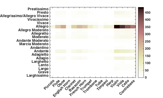
Figure 21. Count of instrument appearances according to tempo.
The sparseness of the data in Figure 21 suggests that 20 tempo terms may be too many. Accordingly, we decided to re-categorize the data into five tempo groups: Very slow (Larghissimo to Larghetto), slow (Adagio to Andantino), moderate (Marcia moderato to Moderato), fast (Allegretto to Allegro), very fast (Vivace to Prestissimo). Figure 22 graphically displays the result of regrouping, normalized for each instrument. It shows that the majority of our samples are still in one of the "fast" tempos. Specifically, 4% of the samples are classified as very slow, 20% as slow, 6% as moderate, 59% as fast, and 11% as very fast. It is important to recall that our method for sampling sonorities allows each page of music to have a roughly equal probability of being sampled. Hypothetical slow and fast movements might both represent five minutes of sounded music. However, the fast movement will necessarily require more pages of musical notation. Consequently, our results should not necessarily be interpreted as indicating that (say) fast passages are three times more common than slow passages. Notice that the question "How much music is fast?" could be interpreted in at least three different ways. One interpretation might be "How much of the elapsed time of music listening involves a fast tempo?" Another interpretation might be "What proportion of musical works/movements tend to exhibit a fast tempo?" A third interpretation might be "What proportion of notated music (i.e. pages) tend to exhibit a fast tempo?" The broad empirical question here is beyond the scope of this study. It should simply be recognized that our tallies reflect sampled pages of notated orchestral music, not the elapsed performance time, nor the proportion of slow or fast works or movements.
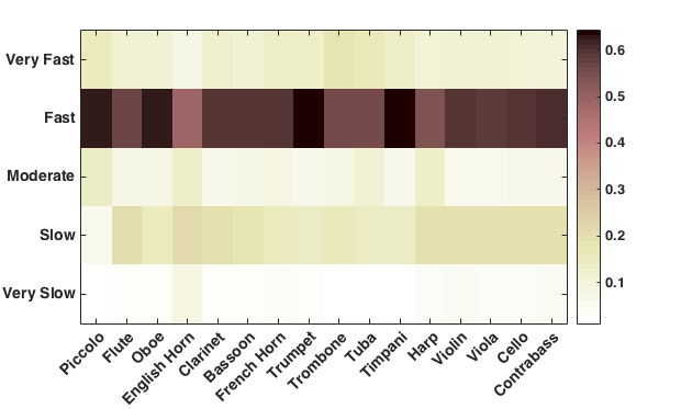
Figure 22. Proportion of samples each instrument is playing for each of five tempo groups (after normalization per instrument).
In Figure 22, timpani and trumpet have cells in the darkest shades (reflecting the highest probability of playing). This means that, when these instruments sound, about 65% of our samples have them performing at a fast tempo. Next darkest cells belong to piccolo and oboe, indicating that they perform at fast tempos for around 60% of our samples. The strings and clarinet, bassoon, French horn, and flute show similar shades that are the next darkest. These instruments belong to the Strings and the Core Winds groups in our clustering analysis, and they tend to sound the most often in orchestral music in general. Trombone, tuba, and harp are the next, and the English horn is the least sounded (still above 40% of time) in a fast tempo.
A comparison of the "Slow" row and the "Fast" rows leads to some pertinent observations. Many instruments (such as clarinet, bassoon, and the strings) tend to show darker shades in both tempos. But there are other instruments that seem to sound more often in one tempo group rather than the other. For example, piccolo, oboe, trumpet, and timpani appear to sound much more frequently in a fast tempo than in slow tempos. However flute, English horn, and harp appear to sound more often in slow and moderate tempos. Of course, these observations should be interpreted carefully, since the number of samples for the "Slow" tempos is much smaller than that for the "Fast" tempos.
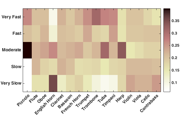
Figure 23. Proportion of samples each instrument is playing for each of five tempo groups (after double normalization; first per tempo, then per instrument).
In light of the dominance of the fast tempos, there is merit to recasting the data using the double normalization procedure used earlier for dynamic levels. The result is shown in Figure 23. Since the first operation treats each tempo as equally likely, it reduces the significant data concentration for the "Fast" tempo. Although this procedure has the potential to highlight otherwise obscure patterns, this procedure exaggerates the effects of small amounts of data, and so warrants caution when interpreting these patterns.
With regard to fast tempos, the greatest affinities are evident in the power instruments—trumpet, trombone, tuba, timpani, and piccolo. With the exception of the trumpet, these power instruments are rarely associated with very slow tempos. Instead, slow tempos are dominated by the strings as well as the notably prominent English horn. In our musical sample, the English horn is almost never present for fast or very fast tempos. The instruments that show the greatest uniformity—spanning a range of tempos—include the Strings and the Core Winds (flute, oboe, clarinet, bassoon, and French horn). As noted, the strings dominate slow and very slow tempos, however the association with slow tempo is notably elevated for the violin, and especially for the contrabass.
In order to discern a more general trend that transcends discrete differences in neighboring cells in Figure 23, we applied a 3-point moving average per instrument. Once again, a cell's value was determined by 60% of its original value and 20% each of its upper and lower neighbors (in the same column) in Figure 23. Figure 24 displays the result. The pattern of instrument/tempo associations clarifies and accords with the observations made for Figure 23: (1) the strings tend to sound rather consistently across all tempos; (2) piccolo, trumpet, trombone, tuba, and timpani sound more often in moderate to faster tempos; (3) other wind instruments (except for the English horn) tend to sound more often in faster tempos, although not as much as piccolo, trumpet, trombone, and tuba do; (4) the English horn tends to sound in a tempo ranging from moderate to very slow; (5) the harp appears equally likely to be used in all tempos, with a possible bias towards moderate tempos.
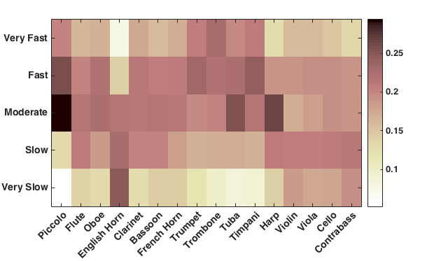
Figure 24. Smoothed (three-point moving average) likelihood proportions of samples each instrument is playing for each of five tempo groups (after double normalization; first per tempo, then per instrument).
Pitch
In our sample, we encoded the pitch of each instrument for each sonority. This allows us to explore possible relationships between pitch and instrument combinations. In the first instance, we might examine the pitch distributions for various instruments. If multiple pitches were recorded for an instrument in a sampled sonority, all the individual pitches were tallied for that instrument. Table 5 identifies the mean, standard deviation, and the highest and lowest pitches found in our samples for each instrument. In addition, the conventional or "textbook" instrument ranges are also included for comparison. Mean values are simple averages of all sampled pitches for the given instrument. In general, the mean pitch in the instrument samples coincides reasonably closely with the center (median) pitch in the conventional instrument range—typically within a distance of 3 semitones. Exceptions include the bass clarinet (6 semitones), contrabassoon (4 semitones), French horn (7 semitones), tuba (6 semitones), timpani (5 semitones), violin (9 semitones), viola (8 semitones), cello (9 semitones), and contrabass (6 semitones). In each of these cases, the mean playing pitch is lower than the conventional median pitch, with the exceptions of French horn and timpani. Note that the mean pitches reported here pertain only to our orchestral sample, whereas the textbook ranges are reported for instruments without regard to context. Ideally, it would be helpful to compare range values for each instrument in both orchestral and non-orchestral contexts. For example, when used in an orchestral ensemble, it may be that the piano tends to function more as a bass or accompaniment instrument, and so account for the seemingly lower pitch range. Unfortunately, we have no pitch range data for non-orchestral repertoires for all of the various instruments, so we do not know whether the mean pitches differ when playing in an orchestral context.
The large differences evident for timpani might arise from the fact that the conventional pitch range has changed over time. In the case of the timpani, drums of different sizes afford different sets of pitches. As the conventional range in Table 5 reflects the lowest pitch of the largest drum and the highest pitch of the smallest drum, the median pitch might not relate to the most frequent pitch of a particular set of timpani. Excluding continuo (as it does not have a conventional pitch range), the mean pitches from our samples and the median pitches from Adler (2002) for the instruments in Table 5 show a very high correlation of +0.95 (p < .001, df = 18).
| Instrument | From sampled data | From Adler (2002) | ||||
|---|---|---|---|---|---|---|
| Mean Pitch | Standard Deviation (semitones) | Lowest Pitch | Highest Pitch | Conventional Sounding Range | Median Pitch | |
| Piccolo | A6 | 6.91 | D♯4 | A♯7 | D5 – C8 | G6 |
| Flute | A5 | 7.42 | A♯3 | D7 | C4 – D7 | G5 |
| Oboe | D♯5 | 5.64 | G♯3 | E6 | A♯3 – G6 | D5 |
| English Horn | G4 | 6.03 | F3 | A♯5 | E3 – C6 | G♯4 |
| Clarinet (B♭) | A4 | 8.00 | G♯2 | F♯6 | D3 – G6 | A♯4 |
| Bass Clarinet | C3 | 10.89 | C♯1 | A♯4 | A♯1 – D5 | F♯3 |
| Bassoon | F♯3 | 8.52 | A♯1 | D♯5 | A♯1 – E5 | G3 |
| Contrabassoon | C2 | 7.52 | B0 | A♯3 | A♯0 – A♯3 | E2 |
| French Horn | C♯4 | 7.23 | D1 | C6 | G1 – F5 | F♯3 |
| Trumpet | A♯4 | 6.40 | G2 | C♯6 | F♯3 – C6 | A4 |
| Trombone | A♯3 | 6.78 | D1 | D5 | E2 – F5 | A♯3 |
| Bass Trombone | C♯3 | 6.15 | C2 | A♯4 | A♯1 – A♯4 | E3 |
| Tuba | E2 | 5.92 | E1 | F♯3 | D1 – G4 | A♯2 |
| Timpani | F♯3 | 11.34 | C2 | A5 | D2 – C4 | C♯3 |
| Piano | D♯4 | 17.40 | C♯1 | G♯7 | A0 – C8 | E4 |
| Continuo | G♯3 | 8.72 | C2 | F5 | N/A | N/A |
| Harp | D3 | 13.74 | D1 | D7 | B1 – F♯7 | D4 |
| Violin | C5 | 8.66 | C3 | A♯7 | G3 – B7 | A5 |
| Viola | D4 | 7.03 | G2 | E6 | C3 – A6 | A♯4 |
| Cello | F3 | 8.59 | C2 | D6 | C2 – E6 | D4 |
| Contrabass | D♯2 | 6.85 | C1 | G♯4 | C1 – G4 | A2 |
Doubling
In any sonority, it is common for certain pitch-classes to be doubled. In ensemble works, it is appropriate to ask which instruments tend to double each other. As before, our focus is on the relationship between unique instruments rather than parts. For example, we will not consider how often two flute parts double each other. Nor will we consider doublings within a part—such as the number of cellos in a cello section. Furthermore, given our random selection of individual sonorities, we necessarily are unable to distinguish momentary doublings from doublings due to shared unison or parallel lines. We simply computed the probability of doubling for every pair of unique instruments playing together in the sampled sonorities. Instruments capable of playing more than one simultaneous pitch raise additional considerations regarding doubling. A single piano chord might suggest that the piano is doubling every instrument in the orchestra. In order to avoid such possibilities, we excluded from consideration all instances where an instrumental part plays two or more pitches. This includes multiple stops played by strings. Finally, it should be noted that two instruments may sometimes contribute more than one type of doubling in a single sonority. Consider a sample with two bassoons playing G♯3 and G♯2 and a tuba playing a G♯2 (we have such a sample in our set). The tuba and the first bassoon manifest an octave doubling, whereas the tuba and the second bassoon manifest a unison doubling. In this case, we counted the same sample once for each category. Table 6 identifies the 22 pairs of instruments that are most likely to perform the same pitch classes, presented in decreasing order of the pitch-class doubling probability. Four data columns are provided for each instrument pair. The second column indicates the total proportion of sonorities where both instruments are present and playing the same pitch class. This probability of pitch-class doubling is further distinguished according to the absolute interval size in the next three columns—unison (third column), octave (fourth column) and two or more octaves (fifth column).
Table 6 shows that the cello and contrabass form the most common doubling pair. When both instruments are sounding, 87% of the sonorities have them performing the same pitch class. The overwhelming majority of this doubling occurs at the interval of an octave.
Two broad trends are evident from Table 6. First, orchestral practice appears to favor within-family doublings (e.g., flute/oboe). Second, there is a greater tendency for doubling among low-pitched instruments (e.g., cello, contrabass, tuba, bassoon, French horn, bassoon, and trombone). Many of these latter doublings involve cross-family pairings (e.g., tuba/contrabass). Doubling of the bass is favored in conventional voice-leading practice (Aarden, 2001). However, another possible influence might relate to blend. Multiple studies have reported that darker timbres blend better with other sounds (Sandell, 1995; Tardieu & McAdams, 2012; Chon & McAdams, 2012). Yet another possibility is that this doubling tendency arises due to critical band spacing. Aarden and von Hippel (2004) have shown that doubling the bass is a natural consequence of spreading out lower pitches in a sonority.
An interesting case involves doubling with the timpani. Although the timpani performs rather sparingly in most compositions, when it does play, it is often doubled by either a trumpet or French horn. With a trumpet, the timpani seems to play equally frequently across the three types of pitch doubling, whereas octave doubling seems to be favored with the French horn. These are likely to be doublings of chord roots, especially the tonic and dominant pitches.
Finally, some readers might wonder why certain popular combinations (such as violin/viola) do not appear in Table 6. In fact, the violin/viola combination was the most observed pairing in our sample set, however, in the majority of sonorities, the two instruments do not engage in pitch-class doubling (56.8%).
| Instrument Combination | Pitch Doubling Probability | |||
|---|---|---|---|---|
| Pitch-class | Unison | Octave | Two or more octaves | |
| Cello / Contrabass | 86.7% | 6.6% | 77.4% | 2.6% |
| Tuba / Contrabass | 84.3% | 63.9% | 20.5% | 0% |
| Bassoon / Tuba | 82.9% | 42.3% | 36.9% | 3.6% |
| Piccolo / Oboe | 82.1% | 0.8% | 54.5% | 26.8% |
| Timpani / Trumpet | 81.8% | 28.7% | 20.6% | 32.5% |
| Trumpet / French Horn | 79.9% | 29.1% | 42.6% | 8.3% |
| Bassoon / Contrabass | 78.6% | 17.4% | 51.0% | 10.2% |
| French horn / Trombone | 78.5% | 45.5% | 30.1% | 2.9% |
| Bassoon / Trombone | 78.4% | 40.9% | 30.1% | 7.5% |
| Flute / Oboe | 78.0% | 27.3% | 48.5% | 2.2% |
| Piccolo / Flute | 74.3% | 22.1% | 47.1% | 5.2% |
| Piccolo / Trombone | 73.9% | 0% | 0% | 73.9% |
| Oboe / Clarinet | 73.8% | 43.2% | 28.7% | 1.9% |
| Oboe / Violin | 73.8% | 45.5% | 27.2% | 1.2% |
| Oboe / Trombone | 73.8% | 1.2% | 38.7% | 33.9% |
| Flute / Clarinet | 73.4% | 15.8% | 46.9% | 10.8% |
| French horn / Timpani | 73.2% | 18.1% | 40.7% | 14.4% |
| Bassoon / Cello | 72.5% | 50.8% | 19.4% | 2.3% |
| Trumpet / Trombone | 71.3% | 12.2% | 46.3% | 12.8% |
| Oboe / Trumpet | 70.9% | 33.3% | 31.4% | 6.2% |
| Oboe / French Horn | 70.8% | 11.1% | 44.3% | 15.5% |
We also carried out a cluster analysis using the pitch-class doubling probability (column 2 of Table 6) for every pair of 16 common orchestral instruments. The results from a Ward linkage with the Euclidean distance are shown in Figure 25.
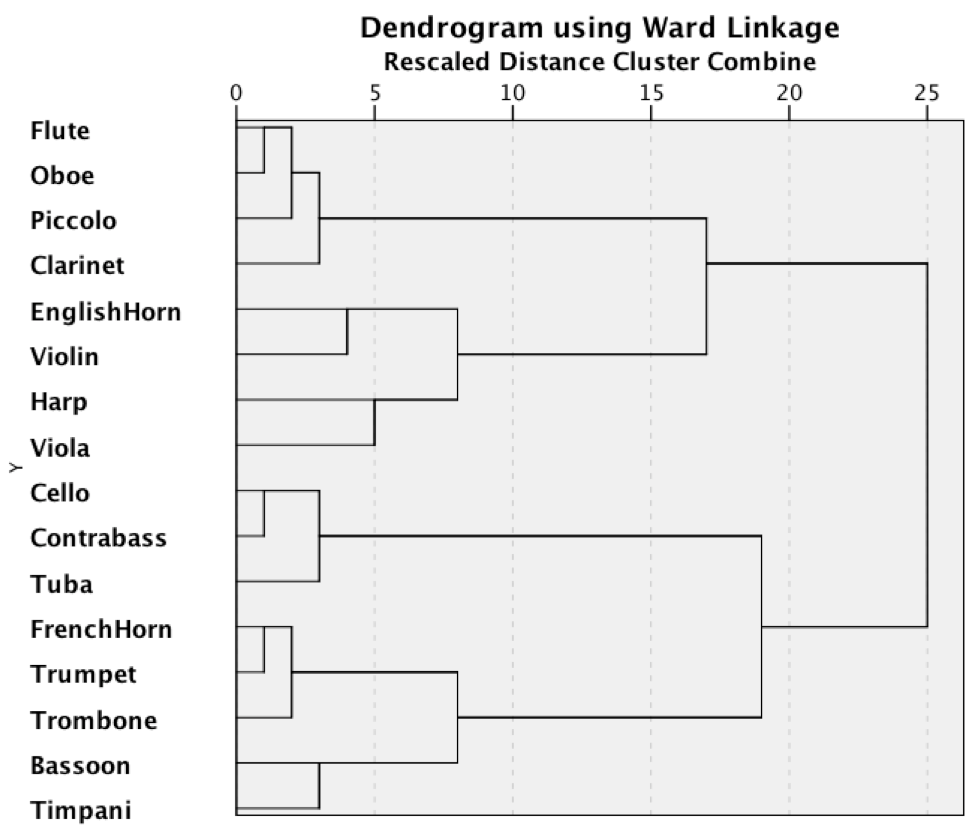
Figure 25. Dendrogram from hierarchical clustering of pitch-class doubling probability.
Before interpreting Figure 25, it is appropriate to consider some of the circumstances under which doublings are likely to occur. One common use of doubling arises when instruments perform the same line, as when doubling a melody line or when two instruments double the bass line. Theoretically, a second form of doubling might arise if certain instruments are thought to be especially suited to playing (say) the third or fifth of a chord. A third consideration relates to the density of the instrumentation. Doublings are likely to increase as the orchestral texture increases in size. Moreover, those instruments that tend to be used only during loud dynamic levels are very likely to end up doubling each other. With these considerations in mind, consider the clustering dendrogram shown in Figure 25.
At the earliest level, we see a close linkage for flute/oboe, cello/contrabass, and French horn/trumpet. In fact, the cello/contrabass doubling is the most often observed from our sample set, for some 87% of the sonorities in which both instruments are sounding. Most of these doublings happen at an octave distance, which is natural considering the pitch ranges of these instruments. The next frequent doubling is seen for contrabass and tuba, which is probably why the tuba is clustered with cello and contrabass. In contrast to the octave-preference in cello/contrabass doubling, the tuba/contrabass doubling occurred mostly at the unison. Note that all three instruments often play the bass line. Bass lines are especially prone to doubling because root position chords are more common than inverted chords. Said another way, bass instruments commonly have less choice of chord factors, and are consequently likely to play the same pitches or pitch-classes.
The French horn/trumpet doubling is the most frequent among the within-brass doublings. When they doubled each other, the octave doubling was used for half of the time. The next highest within-brass doubling is for the French horn/trombone doubling, which favored unison doubling. These differences probably come from the instruments' pitch ranges. Interestingly, these "proto-power" sub-cluster of three brass instruments is combined with the bassoon/timpani sub-cluster, which may form the mid and lower part of "power" passages.
The flute/oboe pair is the second most frequent among the within-woodwind doublings, but they may have been grouped earlier than other frequent pairs of piccolo/flute or piccolo/oboe. These three woodwind instruments appear to form the "melody carrier" among the woodwinds, with frequent support of the clarinet in the same cluster.
Possibly most interesting in Figure 25 is the cluster with English horn/violin and harp/viola. The English horn might have often been used to strengthen the violin as the melody carrier of the string family. On the other hand, the viola often played a supporting role to the violin, in which case the harp might have provided a stronger support with the viola. This cluster could reflect the melody carrying functionality of the string instruments.
In general, the clustering shown in Figure 25 suggests four main doubling patterns. First, doubling appears to be closely linked with instrument families. Notably, woodwinds tend to double woodwinds, and brass tend to double brass. In addition, we see evidence of pitch-range-related doublings. Low instruments (cello, bass), mid instruments (bassoon, trumpet, French horn), and high instruments (flute, oboe) tend to engage in mutual doubling. Finally, there appears to be a strong effect of instrument usage that melody carriers seemed to be grouped together, separate from bass line instruments.
Chord Factors
The notes involved in common tertian chords are distinguished according to their chord position—such as root, third, or fifth. Theorists refer to these tones as chord "factors." Major, minor, diminished, and augmented chords exhibit three factors. In the case of seventh chords, a fourth factor (the seventh) is also distinguished. From the perspective of orchestration, we might consider whether particular instruments tend to be assigned particular chord factors (or whether particular chord factors tend to be assigned to specific instruments). Accordingly, we carried out an appropriate analysis.
We began by employing a script to identify possible candidate chords using the pitch information in the coded sonorities. For the purposes of this analysis we considered only the three most common chord types: the major chord, the minor chord, and the major-minor seventh chord (which often functions as a dominant seventh). For each sonority, we eliminated pitch-class duplicates to produce a unique pitch-class set. In our original coding, transposing instruments were recoded as their untransposed equivalents. In this process, however, pitches were often spelled using an enharmonic equivalent. Consequently, we ignored pitch spelling when identifying the target chords. A "major chord" was deemed to be present when the reduced pitch-class set contained 0, 4, and 7 semitones above any base pitch. Similarly, a "minor chord" was deemed to be present when the reduced pitch-class set contained 0, 3, and 7 semitones above any base pitch. A major-minor seventh chord entailed a pattern 0, 4, 7 and 10 semitones above any base pitch. In identifying a chord as nominally major, minor, or major-minor seventh, all chord factors must be present, and only those factors.
Using this procedure, the complete data set of 1,800 sonorities was reduced to 501 target "chords:" 287 major chords, 159 minor chords, and 55 major-minor seventh chords. For each of these nominal chords, each instrument pitch was classified as either root, third, fifth, or seventh. Table 7 below presents the results for the 19 most commonly sounding instruments. The data in Table 7 have been normalized by dividing each tally by the sum for each column. Hence the values show the proportion of chord factors assigned to a particular instrument. (Columns do not sum to 1.0 because not all instruments are included in the table.) Due to the relatively small amount of data and the problem of multiple tests, we have avoided conducting any statistical tests.
Two levels are visually highlighted in Table 7—identifying values greater than 10% (.10) and values greater than 20% (.20). As might be expected, the strings tend to dominate, simply because they are commonly active. The important question is whether there are associations with particular chord factors.
As might be expected, bass instruments such as the cello, contrabass, and contrabassoon show what appears to be a strong association with chord roots. Similarly, the timpani appears linked to chord roots. Since the majority of chords appear in root position, this would be expected. Interestingly, the cello also shows an elevated association with the third, but only for sonorities equivalent to a minor chord.
The viola exhibits an apparent association with the root and fifth for major chords, the third and fifth for minor chords, and the third, fifth, and seventh for major-minor sevenths.
The violin displays a notable association with the third in the major and minor chords, and the seventh in the major-minor seventh chord. A similar (though not identical) pattern is evident in the oboe. Specifically, the oboe favors the third in major chords, and the third and seventh in major-minor seventh chords. In the case of the major-minor seventh chord, the third and seventh factors are the principal tendency tones requiring specific semitone-movement resolutions. Since many major chords are deployed as dominant functions, the third (seventh scale degree) also exhibits a strong leading or tending quality. Although not as strong, the flute and clarinet exhibit similar associations for the third and seventh factors in the major-minor seventh chord. Finally, we see an apparent association between the fifth of chords and the French horn.
| Major | Minor | Major-minor 7th | ||||||||
|---|---|---|---|---|---|---|---|---|---|---|
| Root | Third | Fifth | Root | Third | Fifth | Root | Third | Fifth | Seventh | |
| Piccolo | 0.01 | 0.00 | 0.01 | 0.01 | 0.01 | 0.01 | 0.01 | 0.01 | 0.01 | 0 |
| Flute | 0.04 | 0.04 | 0.05 | 0.05 | 0.05 | 0.05 | 0.04 | 0.05 | 0.07 | 0.07 |
| Oboe | 0.06 | 0.11 | 0.09 | 0.06 | 0.08 | 0.09 | 0.04 | 0.13 | 0.07 | 0.13 |
| English horn | 0.00 | 0.00 | 0.01 | 0.01 | 0.00 | 0.01 | 0.01 | 0 | 0.01 | 0 |
| Clarinet | 0.04 | 0.05 | 0.06 | 0.03 | 0.06 | 0.07 | 0.04 | 0.07 | 0.08 | 0.08 |
| Bass clarinet | 0.00 | 0.00 | 0 | 0.01 | 0.00 | 0.01 | 0.01 | 0 | 0 | 0.01 |
| Bassoon | 0.07 | 0.06 | 0.06 | 0.06 | 0.08 | 0.05 | 0.07 | 0.06 | 0.08 | 0.05 |
| Contrabassoon | 0.01 | 0.00 | 0.00 | 0.01 | 0 | 0 | 0.01 | 0 | 0 | 0 |
| French horn | 0.07 | 0.08 | 0.09 | 0.06 | 0.04 | 0.09 | 0.10 | 0.09 | 0.13 | 0.09 |
| Trumpet | 0.03 | 0.03 | 0.03 | 0.02 | 0.03 | 0.03 | 0.04 | 0.02 | 0.04 | 0.04 |
| Trombone | 0.02 | 0.04 | 0.03 | 0.02 | 0.02 | 0.03 | 0.02 | 0.02 | 0.01 | 0.03 |
| Bass trombone | 0.01 | 0.00 | 0.01 | 0.02 | 0.01 | 0.00 | 0.02 | 0.01 | 0 | 0 |
| Tuba | 0.01 | 0.00 | 0.00 | 0.02 | 0.01 | 0.01 | 0.01 | 0 | 0 | 0 |
| Timpani | 0.03 | 0.01 | 0.01 | 0.02 | 0.01 | 0.01 | 0.05 | 0 | 0.02 | 0 |
| Harp | 0.01 | 0.01 | 0.01 | 0.01 | 0.01 | 0.01 | 0.01 | 0.02 | 0.01 | 0 |
| Violin | 0.15 | 0.25 | 0.21 | 0.15 | 0.20 | 0.19 | 0.11 | 0.16 | 0.16 | 0.20 |
| Viola | 0.10 | 0.09 | 0.15 | 0.09 | 0.11 | 0.17 | 0.08 | 0.14 | 0.12 | 0.12 |
| Cello | 0.12 | 0.05 | 0.07 | 0.13 | 0.10 | 0.06 | 0.11 | 0.08 | 0.05 | 0.06 |
| Contrabass | 0.12 | 0.05 | 0.03 | 0.12 | 0.07 | 0.01 | 0.11 | 0.05 | 0.02 | 0.03 |
Pitch, Loudness, and Tempo Interactions
Existing research has identified environmental, perceptual, and cognitive associations between pitch, tempo, and dynamic level. With regard to pitch and dynamics, Sundberg et al. (1983) have noted that "In almost every musical instrument, the amplitude increases somewhat with the fundamental frequency." This association has been dubbed the "high-loud rule" by Friberg et al. (2006). Indeed, the word "alto" in Italian, Spanish and Portuguese means both high and loud (Eitan, 2013).
In the case of dynamics and tempo, Kohn and Eitan (2009) have shown that listeners rate loud performances as sounding faster than quieter performances of the same music. Eitan and his colleagues have demonstrated this association in musician and non-musician adults (Eitan & Granot, 2006), children (Tubul, 2010), and in congenitally blind adults (Eitan et al., 2012).
In the case of pitch and tempo, Broze and Huron (2013) employed several contrasting methods and documented a ubiquitous "higher is faster" association in music. Related to this association, Friberg et al. (2006), have also observed that music performances sound better when ascending pitch sequences increase in tempo. Using an analysis-by-synthesis approach, they found that an optimum musical effect occurs when the duration of each note is decreased by 3% if the ensuing note is higher in pitch. The authors dubbed this the "faster uphill" rule (2006).
By way of summary, fast tempo, high pitch, and loud dynamics all appear to be positively correlated. This raises the question as to whether such associations can also be observed in our sample of orchestral sonorities. Accordingly, we carried out additional analyses.
With regard to possible associations between pitch height and dynamic level, for each instrument, we correlated the pitch information (in MIDI numbers) with the associated dynamic level, where dynamics were treated as rank-ordered data (1 corresponding to pppp and 10 corresponding to ffff). We then calculated Spearman's rank-order correlation for each instrument. A positive correlation suggests that the instrument tends to play higher in pitch when the dynamic level is louder. Conversely, a negative correlation implies that the instrument tends to play lower in pitch when the dynamic level is higher. Table 8 presents the results for 21 of the 91 orchestral instruments, where the p values are less than 0.1. We have presented the results sorted according to increasing p values rather than by the correlation magnitudes in order to reduce the tendency to over-interpreting spurious (insignificant) high correlation values. Significant results at p = .05 level (top 15 rows) are presented in bold fonts with a preceding asterisk. No correction has been made for multiple tests. Note that all correlation coefficients are negative values with two exceptions of bassoon and harpsichord. This suggests that if any pattern exists between pitch height and dynamic level, it favors a lower-louder association rather than a higher-louder association. In order to test the generality of this result, one might consider aggregating all of the data and performing a single test across all instruments. For example, a Spearman's rank order correlation on this entire set of pitch-dynamics data yields rS = −.08 (p < .001). However, in order to amalgamate the data, it is appropriate first to adjust for the different instrument ranges. Accordingly, we normalized the sampled pitches for each instrument and then calculated Spearman's rank-order correlation between the ordinal dynamic level data and the normalized pitch. The result is very a mild negative correlation of −0.12 (p < .001). The corresponding R2 is 0.0156. This suggests that there is no systematic tendency to play higher pitches using a louder dynamic.
| Instrument | rS | p | df |
|---|---|---|---|
| * Viola | −.24 | < .001 | 1392 |
| * Flute | −.29 | < .001 | 822 |
| * Clarinet | −.28 | < .001 | 888 |
| * Violin | −.15 | < .001 | 2881 |
| * French horn | −.12 | < .001 | 1399 |
| * Cello | −.12 | < .001 | 1195 |
| * Trombone | −.17 | < .001 | 367 |
| * Bassoon | .09 | < .005 | 1038 |
| * Timpani | −.17 | < .005 | 294 |
| * Trumpet | −.11 | < .01 | 553 |
| * Oboe | −.07 | < .05 | 1022 |
| * Vibraphone | −.58 | < .05 | 12 |
| * Bongo | −.21 | < .05 | 105 |
| * Trumpet in D | −.77 | < .05 | 6 |
| * Harp | −.10 | < .05 | 369 |
| Clarini | −.59 | .0566 | 9 |
| Contrabass | −.06 | .0640 | 885 |
| Alto Saxophone | .79 | .0714 | 5 |
| Tubular bells | −.73 | .0762 | 5 |
| Mandolin | −.76 | .0952 | 5 |
| Harpsichord | .10 | .0974 | 266 |
Similarly, we investigated whether any relationship might exist between pitch and tempo. Table 9 reports the various pitch/tempo correlations in ascending order of the significance value (showing only values under .1). Positive correlations suggest that the instrument tends to play higher in pitch when the tempo is faster. At first glance, the preponderance of positive correlations in this table suggests there may be some relationship. However, considering the entire set of pitch/tempo data set, the hypothesized positive correlation was found but in a very small magnitude, rS (11074) = .05, p < .001. After adjusting for instrument range, we once again amalgamated all of the data and tested for a general association. The result was still a tiny correlation of 0.06 (p < .001). The corresponding R2 is a miniscule 0.004. The result implies that there is no systematic tendency to play higher pitches using a faster tempo.
| Instrument | rS | p | df |
|---|---|---|---|
| * Violin | .07 | < .001 | 2234 |
| * Flute | .14 | < .001 | 615 |
| * Timpani | .19 | < .01 | 209 |
| * Bongo | .30 | < .01 | 77 |
| * French horn | .08 | < .01 | 1017 |
| * Organ | −.35 | < .05 | 48 |
| * Contrabassoon | .40 | < .05 | 34 |
| * Cello | .07 | < .05 | 922 |
| * Clarinet | .09 | < .05 | 643 |
| * Piano | .16 | < .05 | 161 |
| * Alto Saxophone | .75 | < .05 | 6 |
| Bass Trombone | −.24 | .0545 | 65 |
| Harp | .12 | .0832 | 201 |
| Instrument | rS | p | df |
|---|---|---|---|
| * Violin | −.25 | < .001 | 1650 |
| * French horn | −.29 | < .001 | 903 |
| * Viola | −.25 | < .001 | 758 |
| * Oboe | −.24 | < .001 | 721 |
| * Clarinet | −.27 | < .001 | 556 |
| * Cello | −.23 | < .001 | 718 |
| * Continuo | −.48 | < .001 | 132 |
| * Contrabass | −.24 | < .001 | 555 |
| * Flute | −.24 | < .001 | 544 |
| * Bassoon | −.22 | < .001 | 672 |
| * Harpsichord | −.49 | < .001 | 96 |
| * Timpani | −.35 | < .001 | 191 |
| * Bongo | −.51 | < .001 | 74 |
| * Ventilhorn | −.97 | < .001 | 8 |
| * Trumpet | −.21 | < .001 | 326 |
| * Trombone | −.26 | < .001 | 198 |
| * Contrabassoon | −.53 | < .005 | 28 |
| * English horn | −.32 | < .05 | 53 |
| * Harp | −.25 | < .05 | 69 |
| Tuba | −.24 | .0828 | 51 |
| Snare drum | −.45 | .0836 | 14 |
In the same manner, we examined possible relationships between tempo and dynamics. Table 10 displays the various tempo/dynamics correlations in ascending order of the significance value (showing only values under .1). Note that all instruments listed in this table show negative correlations, suggesting that they tend to play louder dynamics in slower tempos and/or quieter dynamics in faster tempos. In fact, the tempo/dynamics samples obtained from all 91 instruments exhibited this negative relationship, rS (8736) = −.24, p < .001. Our results here are contrary to those reported by Eitan and his colleagues. We have no explanation for this discrepancy. Perhaps the composers in our sample somehow aimed to surprise listeners by doing the opposite of what seems natural (that the louder performance is perceived as faster or vice versa).
A close examination of the list of instruments in Table 10 shows us that all four string instruments are included as well as the instruments in the Core Winds group (bassoon, clarinet, flute, oboe, and French horn). Some of the large correlation values may be spurious due to the very limited number of samples (e.g., Ventilhorn).
DISCUSSION
In this study we examined patterns of instrumentation in Western orchestral music composed between 1701 and 2000. Some 1,800 sounding moments (sonorities) were sampled from 180 orchestral works by 147 composers. These sonorities included 91 unique instruments distributed across 165 notated parts. The sample was stratified so that equivalent numbers of samples were drawn from each of six 50-year epochs. We examined changes of instrumentation and instrument usage, changes in ensemble size, common instrument combinations, instrument groupings or clusterings and their changes over time, the association of different instruments with various dynamic levels and with different tempos, prevalent instrument pitch ranges, pitch-related doublings, affinities for chord factors, and possible pitch/dynamics/tempo interactions.
In summarizing the various findings from our study, it is appropriate to begin by reminding readers of various limitations and caveats. First, our sample size of 1,800 sonorities is tiny in comparison to the millions of orchestral sonorities composed over the 300-year target period. Although care was taken to assemble representative samples, various biases are inescapable. We made no effort to identify urtext scores, so the results—especially with regard to dynamic markings—are potentially confounded by subsequent editorial interventions. Nor did we endeavor to normalize or compensate for possible changes in baseline dynamic levels over the period spanned by the study. (Recall that according to Ladinig and Huron dynamic markings in keyboard music became notably quieter between the 18th and late 19th centuries.) With regard to tempo markings, we have assumed that markings such as Andante and Allegro hold broadly similar meanings over the three centuries spanned by the study. As noted earlier, the instrumentation specified in a score does not necessarily reflect actual performance practices. Especially in Baroque and earlier music, instrumentation was frequently supplemented or altered by the performers (Harnoncourt, 1988, p. 160; Weaver, 2006, p. 28). Finally, we should note that the goal of data independence was compromised by sampling 10 sonorities from each work rather than only a single sonority from each work (although in fairness, most works involved multiple movements, so the sampled sonorities are more independent than might otherwise be apparent). All of these caveats suggest that the findings be interpreted with appropriate caution.
As an exploratory study, we did not approach the data with any a priori hypotheses. Consequently, all of our observations and interpretations are post hoc. Given the wide range and large number of observations, we limited the number of statistical tests in order to minimize the problem of multiple tests. Nevertheless, even informal observations invite the problem of multiple tests (Huron, 2013). Given the sample size and the large number of observations made, correcting for multiple tests would be expected to result in few statistically significant observations. Consequently, most of our observations are best regarded as suggestive.
Many of our results will necessarily be considered unexceptional because they confirm widespread musical intuitions and observations made using less formal approaches (e.g., Harnoncourt, 1988; Stauffer, 2006; Weaver, 2006; Dolan, 2014). On the one hand, our results provide independent converging evidence for these views. At the same time, we can point to a considerable number of novel observations.
With regard to ensemble size, our study provides no direct index of the total number of instruments performing a given work. Nevertheless, the number of notated parts provides a telling correlate of ensemble size. Orchestral scores in the early 18th century contain an average of 7–8 notated parts. The number of notated parts increased continuously to the beginning of the 20th century when the average number of parts in our sample rises to 33 (ranging between 5 and 52). However, no further increase in the ensemble of parts occurred in the latter half of the 20th century, while there remained a considerable range of ensemble sizes.
In general, string instruments dominate both instrumentation and sounding sonorities (see Figures 1 and 6, and Tables 2 and 3). The most common instrument combination for our entire sample is the five-part string consort consisting of first and second violins, viola, cello, and contrabass. The next most common combinations across all epochs studied include various combinations and permutations of string instruments. Of the four string instruments, the violin plays most frequently, followed by the viola and cello (roughly equivalent usage), followed by the contrabass.
Of course, the centrality of the violin family (violin, viola, and cello) has long been observed by musicologists (e.g., Stauffer, 2006, p. 41). In accounting for the prominence of the violin family in orchestral practice, Weaver (2006, pp. 10–11) suggests four principal factors. First, in contrast with plucked string instruments (such as the lute), the instruments of the violin family are able to sustain tones for an arbitrary length of time. Second, violin family instruments are better able to vary loudness, especially when compared with capped reed instruments like crumhorns. Third, pitch is more easily varied with instruments of the violin family. This is most notable when contrasting these instruments with woodwinds and brass instruments. Fourth, compared with the (moveable fret) viol family, members of the violin family are easier to tune.
There are additional advantages. Compared with the pre-valve brass and pre-Boehm woodwinds, it is easier for string instrument to play in a wide range of keys. Finally, the violin family spans a very wide pitch range while maintaining remarkably similar timbres that facilitate ensemble blend (Harnoncourt, 1988). The viol family might have rivaled the violin family as the preeminent members of the orchestra, however their softer timbre and difficulty of tuning was probably decisive in their decline. The only viol instrument to remain in the orchestra is the contrabass—with the moveable frets removed.
The dominance of the strings notwithstanding, our sample of music also testifies to the widely observed decline in string usage over time. Although the strings are nearly ubiquitous members of the instrumentation, their presence in any given sonority has declined from around 85% in the early 18th century, to around 60% in the late 20th century (see Figure 1).
As expected, over time the use of the harpsichord declined (Figure 4), whereas the clarinet became more prominent (Figure 2). In the 18th century, the clarinet initially appears as part of a cluster deemed Effects (Figure 9), however by the 19th century, the clarinet has joined a cluster deemed Core Winds (Figure 10). The oboe was the most popularly included woodwind instrument in the 18th century. After 1800, flute, oboe, clarinet and bassoon are roughly equivalent in use, although clarinet and bassoon sound more often than flute and oboe (Figure 2). When present, the bassoon has tended to be the most active of all woodwinds. Throughout all periods, the French horn is the preeminent brass instrument (Figure 3). Throughout the late 19th century, the timpani was present in nearly all orchestral works we sampled (Figure 4).
When the piano is included in the instrumentation, its usage declines dramatically from the early 19th century to the mid 20th century. That usage trend reverses in the late 20th century. Notice also that by the late 20th century, the piano is as frequently included in orchestral score as was the harpsichord in the early 18th century (Figure 4).
In considering instrument groupings, we considered three models: (1) the instrument family model (Strings-Woodwinds-Brass-Percussion), (2) Johnson's Standard-Power-Color model, and (3) the results of our own cluster analysis, the Strings-Core Winds-Effects model. Using the same 19 instruments analyzed by Johnson, our cluster analyses of paired instrument associations produced the same three robust clusters in each of the 18th, 19th, and 20th centuries. One cluster (deemed Strings) consists of the violin, viola, cello, and contrabass. A second cluster (deemed Core Winds) consists of flute, oboe, clarinet, bassoon, and French horn. A final cluster (deemed Effects) includes piccolo, English horn, bass clarinet, contrabassoon, trumpet, cornet, trombone, tuba, harp, and timpani.
Apart from the addition of the French horn, our Strings and Core Winds groups correspond to Johnson's Standard instrument cluster. Our Effects cluster appears to be an amalgamation of two of Johnson's clusters: the Power instruments (piccolo, trumpet, trombone, French horn, tuba, timpani), and the Color instruments (English horn, cornet, harp, bass clarinet, contrabassoon). It should be noted that the musical sample used in our study is three times larger than the sample used in Johnson's study.
In tracing historical changes in instrument groupings, we made use of all three models. The models all exhibited parallel historical patterns (Figures 13, 14, and 15). Consistent with informal historical observations, there is a rapid increase in novel instrument combinations and a concomitant rapid reduction in the mutual association of common instrument groupings such as the Strings family and Johnson's Standard instruments. This reduction is most apparent in the 18th century. The rate of decline abates somewhat in the 19th century. However, there remains a concurrent modest increase in the cohesion of other groups (woodwinds/brass/power/effects instruments) over the 18th and 19th centuries. Once again, these changes agree with traditional historical observations that successive generations of composers continued to pursue novel sounds, both by incorporating new instruments into the ensemble, and by using new instrument combinations.
Turning to some of the sub-cluster patterns, in the 18th century, the oboe stands apart from the other Core Winds, consistent with the oboe's preeminence in that century (Figure 9). By the 19th and 20th centuries, sub-clusters of the Core Winds suggest separate groupings of higher-pitched instruments (flute, oboe) from lower-pitched instruments (bassoon, French horn) with the clarinet vacillating between the two (Figures 10 & 11).
With regard to the Strings cluster, two sub-clusters are evident throughout the 18th and 19th centuries. In the 18th century, cello and contrabass form one sub-cluster, with violin and viola forming a second sub-cluster (Figure 9). By contrast, in the 19th century, the cello is grouped with violin and viola, while the contrabass forms its own separate cluster (Figure 10). It is possible that the yoking together of cello and contrabass in the 18th century is a legacy of basso-continuo practice. In the 19th century, rather than simply constantly doubling the cello, the contrabass appears to have achieved considerable functional independence. Although the contrabass has a strong tendency to double the same pitch chromas as the cello, later composers are more sparing in their use of the contrabass, choosing particular occasions for such doubling rather than automatically doubling the cellos (Figure 11).
The Effects cluster is something of a grab-bag. In the 18th century, there is no evidence of any sub-clustering (Figure 9). By the 19th century, two main sub-clusters are evident. One sub-cluster entails trumpet, trombone, and timpani—suggesting what might be regarded as a "proto-power" group (Figure 10). The 20th-century version of this "proto-power" sub-cluster appears to consist of tuba, trombone, contrabassoon and timpani, plus the harp. With the exception of the harp, this proto-power sub-cluster emphasizes low-and-loud instrumentation. In contrast with Johnson's Power group, the trumpet and piccolo have been assigned to a different sub-cluster that contains other instruments more reminiscent of Johnson's Color group. This regrouping implies that the "power" sound in the 20th century emphasizes a darker overall texture compared with earlier centuries (Figure 11). In their corpus study of 18th and 19th century classical music, Horn and Huron (2012) observed a marked decline in "light/effervescent" and "joyful" musics, and a concomitant increase in "passionate" and "serious" musics. The low-loud power pattern observed here suggests a possible continuity towards more serious or dark musical expressions.
Apart from the clustering of instruments into mutually associated groups, we also directly examined the novelty of instrument combinations over history. Specifically, we observed a marked rise in instrument-combination entropy from the beginning of the 18th century to the early-middle 20th century. However, we also observed an unexpected large drop in entropy in the late 20th century (Figure 16). The drop was dramatic, suggesting that the novelty of instrument combinations declined to values lower than found throughout the 19th century. In other words, the results imply that the number of unique combinations of instruments declined dramatically in the late 20th century.
In reconciling the historical analyses of instrument clusters with the entropy measures, we have suggested that the late 20th century composers may have made use of stable-repeated combinations of instruments, but that these combinations do not coincide with traditional instrument groupings, such as by instrument family. That is, orchestration in the late 20th century appears to be characterized by a form of predictable uniqueness or standardized novelty. Further work is warranted in order to determine whether these observations arise from stereotypical use of instruments within individual compositions, or shared "stereotypical novelty" across compositions.
With regard to dynamic levels, many of our observations reinforce common musical intuitions. For example, woodwinds and brass tend to be associated with louder dynamics whereas strings tend to be associated with quieter dynamics (Figure 17). Loud dynamic levels are especially likely to involve the piccolo and timpani, moderate dynamics tend to favor the bassoon, and quiet dynamics tend to be associated with flute and French horn. Other observations are less obvious. Interestingly, the harp exhibits a strong association with f (Figure 18). The timpani, contrabass, and (to a less extent) flute exhibit a marked bifurcation: they are associated with both ff and pp passages (Figure 19). The timpani in particular rarely plays during more moderate dynamic levels. We expect that a larger sample might show that the harp is also associated with quiet passages, and so the harp might exhibit the same dynamic bifurcation seen in the timpani and contrabass.
In the case of changing dynamics, crescendos are significantly more common than decrescendos (Figure 17). This pattern is not restricted to orchestral music. Huron (1990a, 1990b, 1991) has observed a general tendency for crescendos to be significantly longer in duration than diminuendos, and that sudden changes of dynamics tend to reduce the loudness (e.g., subito piano rather than subito forte). Huron (1991) notes that these dynamic patterns are consistent with known principles for attracting listener attention.
In orchestral works, the French horn and harp tend to be associated with diminuendos, whereas the English horn tends to be associated with crescendos (Figure 19). However, changing dynamic levels are most strongly associated with the clarinet—both crescendos and diminuendos. In general, dynamic changes appear to have an association with pitch height: louder-higher and quieter-lower. Hence the piccolo, flute, and oboe have a greater affinity for crescendos, whereas the clarinet, French horn, and tuba have a greater affinity for diminuendos (Figure 19).
With respect to tempo, the strings tend to sound rather consistently across all tempos, By contrast, power instruments such as the piccolo, trumpet, trombone, tuba, and timpani sound more often in moderate to faster tempos. The English horn appears to have a special affinity for slow or very slow tempos. With the exception of the English horn, the other wind instruments tend to favor faster passages; however they do not exhibit the marked affinity for fast tempos found in piccolo, trumpet, trombone, and tuba. The harp appears equally likely to be used in all tempos, with a possible bias towards moderate tempos (Figure 24).
With regard to pitch, the distribution of pitches for the various instruments coincides well with conventional instrument ranges described by Adler (2002) (Table 4). This implies—but does not establish—that the sounding pitch ranges for various instruments change little over time when playing in an orchestral context.
A common feature of orchestration is instrument doubling, where two or more instruments play either the same pitch (unison) or duplicate pitch-classes at the distance of one or more octaves. With regard to doubling, the cello and contrabass exhibit the closest alliance of all instrument pairings (Table 6). We also observed many incidents of doublings within an instrument family or doublings of low-pitched instruments. Finally, there are close doublings found among timpani, trumpet, trombone, piccolo, and French horn. All these instruments are classified by Johnson as Power instruments. In our cluster analysis, they belong to the Effects cluster, except for the French horn in the Core Winds cluster.
Broadly speaking, pitch range and instrument family appear to play a role in pitch-class doubling. With regard to the pitch range, high-pitched instruments tend to double other high-pitched instruments (flute, oboe); similarly mid-pitched instruments (trumpet, French horn) and low-pitched instruments (cello, contrabass) tend to double instruments in the same pitch region. With the exception of the strings, doubling also appears to be linked with instrument families: woodwinds tend to double woodwinds, and brass tend to double brass (Figure 25).
When viewed from the perspective of chord factor, bass instruments such as the contrabass, contrabassoon, cello, and timpani are (not surprisingly) strongly associated with chord roots (Table 7). In the case of the minor chord, the cello also exhibits an elevated association with the third. The French horn tends to favor the fifth of chords. The viola exhibits an apparent association with the root and fifth for major chords, the third and fifth for minor chords, and the third, fifth, and seventh for major-minor sevenths (Table 7).
The oboe displays a notable association with the third in major chords, and with the third and seventh in major-minor seventh chords. The violin shares these same dispositions, but adds an association with the third in minor chords as well. In general, tendency tones (such as the third and seventh in the major-minor seventh chord) are likely to be assigned to high-pitched instruments, notably the violin and the oboe, and to a lesser extent, the flute and clarinet (Table 7).
With regard to possible pitch-tempo and pitch-dynamic interactions, we found no notable tendencies. Although other studies have revealed a general tendency for instruments to play high pitches with a louder dynamic, we found no such general association between pitch and dynamic level in our orchestral sample. Similarly, although there is a general musical tendency for high tones to be associated with a faster tempo, we found no general association between tempo and pitch.
In this study, we have made a number of general observations regarding patterns of orchestration. It bears emphasizing that our study has painted a picture using only broad brush strokes. In light of the breadth of our musical sample, the descriptions offered here merely represent some of the typical or commonplace orchestration practices. Nevertheless, these descriptions provide something of a normative background against which the orchestration practices of individual composers, different regions or nationalities, might be characterized.
ACKNOWLEDGEMENTS
This article was copyedited by Tanushree Agrawal and layout edited by Kelly Jakubowski.
NOTES
-
Correspondence can be addressed to Song Hui Chon at songhui.chon@rit.edu.
Return to Text -
https://en.wikipedia.org/wiki/List_of_classical_music_composers_by_era last accessed July 18, 2015.
Return to Text -
As of September 1, 2015.
Return to Text -
http://imslp.org as of August 17, 2015.
Return to Text -
http://en.wikipedia.org/wiki/Tempo last accessed September 1, 2015.
Return to Text
REFERENCES
- Aarden, B. (2001). An empirical study of chord-tone doubling in common era music. Master's Thesis, School of Music, Ohio State University.
- Aarden, B. & von Hippel, P.T. (2004). Rules of chord doubling (and spacing): Which ones do we need? Music Theory Online, 10(2). http://mto.societymusictheory.org/issues/mto.04.10.2/mto.04.10.2.aarden_hippel_frames.html.
- Adler, S. (2002). The Study of Orchestration. New York: W.W. Norton.
- Berlioz, L.H. (1855). Berlioz's orchestration treatise: A translation and commentary (Cambridge musical texts and monographs) (H. Macdonald, Ed.). Cambridge, England: Cambridge University Press. (Republished in 2002).
- Blatter, A. (1980). Instrumentation and Orchestration. New York: Schirmer.
- Broze, Y. & Huron, D. (2013). Is higher music faster? A pitch-speed relationship in music. Music Perception, 31(1). https://doi.org/10.1525/mp.2013.31.1.19
- Caclin, A., McAdams, S., Smith, B. K., & Winsberg, S. (2005). Acoustic correlates of timbre space dimensions: A confirmatory study using synthetic tones. Journal of the Acoustical Society of America, 118(1), 471–482. https://doi.org/10.1121/1.1929229
- Chon, S.H. & McAdams, S. (2012). Exploring Blending as a Function of Timbre Saliency, In Proceedings of the 12th International Conference of Music Perception and Cognition (ICMPC), Thessaloniki, Greece, pp. 222–223.
- Dolan, E.I. (2014). The Orchestral Revolution: Haydn and the Technologies of Timbre. Cambridge: Cambridge University Press.
- Dubal, D. (2001). The Essential Canon of Classical Music. New York: North Point Press.
- Eitan, Z. (2013). How pitch and loudness shape musical space and motion. In S-L. Tan, A.J. Cohen, S.D. Lipscomb & R.A. Kendall (Eds.), The Psychology of Music in Multimedia. Oxford: Oxford University Press, 165–191. https://doi.org/10.1093/acprof:oso/9780199608157.003.0008
- Eitan, Z. & Granot, R.Y. (2006). How music moves. Music Perception, 23(3), 221–248. https://doi.org/10.1525/mp.2006.23.3.221
- Eitan, Z., Ornoy, E., & Granot, R.Y. (2012). Listening in the dark: Congenital and early blindness and cross-domain mappings in music. Psychomusicology: Music, Mind, and Brain, 22(1), 33–45. https://doi.org/10.1037/a0028939
- Friberg, A., Bresin, R., & Sundberg, J. (2006). Overview of the KTH rule system for musical performance. Advances in Cognitive Psychology, 2(2–3), 145–161. https://doi.org/10.2478/v10053-008-0052-x
- Forsyth, C. (1914). Orchestration. London: Macmillan.
- Gevaert, F.-A. (1885). Nouveau traité d'instrumentation, Paris, Bruxelles: Lemoine & fils.
- Grey, J.M. (1977). Multidimensional perceptual scaling of musical timbres. Journal of the Acoustical Society of America, 61(5), 1270–1277. https://doi.org/10.1121/1.381428
- Grey, J.M., & Gordon, J.W. (1978). Perceptual effects of spectral modifications on musical timbres. Journal of the Acoustical Society of America, 63, 1493–1500. https://doi.org/10.1121/1.381843
- Harnoncourt, N. (1988). Baroque music today: Music as speech: Ways to a new understanding of music (R.G. Pauly, Trans.). Portland, Oregon: Amadeus Press.
- Horn, K. & Huron D. (2012). Major and minor: An empricial study of the transition between Classicism and Romanticism. In E. Cambouropoulos, C. Tsougras, P. Mavromatis & K. Pastiadis (editors), Proceedings of the 12th International Conference on Music Perception and Cognition. Thessaloniki, Greece: ESCOM, pp.456–464.
- Huron, D. (1990a). Crescendo/Diminuendo asymmetries in Beethoven's piano sonatas. Music Perception, 7(4), 395–402. https://doi.org/10.2307/40285475
- Huron, D. (1990b). Increment/Decrement asymmetries in polyphonic sonorities. Music Perception, 7(4), 385–393. https://doi.org/10.2307/40285474
- Huron, D. (1991). The ramp archetype: A study of musical dynamics in 14 piano composers. Psychology of Music, 19(1), 33–45. https://doi.org/10.1177/0305735691191003
- Huron, D. (2013). On the virtuous and the vexatious in an age of big data. Music Perception, 31(1), 4–9. https://doi.org/10.1525/mp.2013.31.1.4
- Johnson, R. (2007). Towards a theory of orchestration: A quantitative study of instrumental combinations in Romantic-era symphonic works. Master's thesis, School of Music, Ohio State University.
- Johnson, R. (2011). The Standard, Power, and Color model of instrument combination in Romantic-era symphonic works. Empirical Musicology Review, 6(1), 2–19. https://doi.org/10.18061/1811/49759
- Jolly, J. (2010). The Gramophone Classical Music Guide. Haymarket Consumer Media.
- Kendall, R.A., & Carterette, E.C. (1993). Identification and blend of timbres as a basis for orchestration Contemporary Music Review, 9(1–2), 51–67. https://doi.org/10.1080/07494469300640341
- Kendall, R.A., Carterette, E.C., & Hajda, J.M. (1999). Perceptual and acoustical features of natural and synthetic orchestral Instrument tones. Music Perception, 16(3), 327–363. https://doi.org/10.2307/40285796
- Kennan, K. (1952). The Technique of Orchestration. Englewood Cliffs, New Jersey: Prentice-Hall.
- Koechlin, C. (1954-9). Traité de l'orchestration: en quatre volumes. Paris: M. Eschig.
- Kohn, D., & Eitan, Z. (2009). Musical parameters and children's movement responses. In J. Louhivuori, T. Eerola, S. Saarikallio, T. Himberg, P-S. Eerola (Eds.) Proceedings of the 7th Triennial Conference of European Society for the Cognitive Sciences of Music. Jyväskylä, Finland, pp. 233–241.
- Krumhansl, C.L. (1989). Why is musical timbre so hard to understand? In S. Nielzen & O. Olsson (Eds.), Structure and perception of electroacoustic sound and music (pp. 44–53). Amsterdam: Excerpta Medica.
- Ladinig, O. & Huron, D. (2010). Dynamic levels in Classical and Romantic keyboard music: Effect of musical mode. Empirical Musicology Review, 5(2), 51–56. https://doi.org/10.18061/1811/46762
- Lakatos, S. (2000). A common perceptual space for harmonic and percussive timbres. Perception & Psychophysics, 62(7), 1426–1439. https://doi.org/10.3758/BF03212144
- McAdams, S. (2003). Perception of musical timbre. Bulletin of Psychology and the Arts, 4, 39–42.
- McAdams, S., Winsberg, S., Donnadieu, S., De Soete, G., & Krimphoff, J. (1995). Perceptual scaling of synthesized musical timbres: Common dimensions, specificities, and latent subject classes. Psychological Research, 58, 177–192. https://doi.org/10.1007/BF00419633
- Piston, W. (1955). Orchestration. New York: W.W. Norton.
- Rimsky-Korsakov, N. (1964). Principles of Orchestration. Edited by Maximilian Steinberg. English translation by Edward Agate New York: Dover Publications. (Original work published 1912)
- Sandell, G.J. (1991). Concurrent timbres in orchestration: A perceptual study of factors determining "blend". Ph.D. dissertation, School of Music, Northwestern University.
- Sandell, G.J. (1995). Roles for spectral centroid and other factors in determining "blended" instrument pairings in orchestration. Music Perception, 13, 209–246. https://doi.org/10.2307/40285694
- Sandell, G.J., & Martens, W.L. (1995). Perceptual evaluation of principal-component-based synthesis of musical timbres. Journal of the Audio Engineering Society, 43(12), 1013–1028.
- Sevsay, E. (2013). The Cambridge Guide to Orchestration. Cambridge: Cambridge University Press.
- Shannon C.E., & Weaver W. (1949). The Mathematical Theory of Communication. London and New York: University of Illinois Press.
- Stauffer, G.B. (2006). The modern orchestra: A creation of the late eighteenth century. In J. Peyser (ed.), The Orchestra (pp. 41–72). Milwaukee, WI: Hal Leonard.
- Sundberg, J., Askenfelt, A., & and Frydén, L. (1983). Musical performance: A synthesis-by-rule approach. Computer Music Journal, 7(1), 37–43. https://doi.org/10.2307/3679917
- Tardieu, D., & McAdams, S. (2012). Perception of dyads of impulsive and sustained sounds. Music Perception, 30(2), 117–128. https://doi.org/10.1525/mp.2012.30.2.117
- Tubul, Z.E.N. (2010). Musical parameters and children's images of motion. Musicae Scientiae, 14(2), 89–111. https://doi.org/10.1177/10298649100140S207
- Weaver, R.L. (2006). The Consolidation of the main elements of the orchestra: 1470-1768. In J. Peyser (ed.), The Orchestra (pp. 7–40). Milwaukee, WI: Hal Leonard.
- Widor, C.-M. (1906) Technique de lâ orchestre moderne. Paris, 1904. Translated by Edward Suddard as: The technique of the modern orchestra: A manual of practical instrumentation. London, J. Williams, 1906.
